
As the automotive industry continues to evolve towards new energy solutions, the battery electric car has become a focal point of technological advancement. Ensuring the safe operation of battery electric cars is paramount, and fault diagnosis in battery systems is a critical research and production issue. Battery faults, such as internal short circuits (ISC), can lead to severe safety incidents like thermal runaway. Most existing fault detection methods rely on laboratory data, lacking validation with real-world operating data from battery electric cars. To address practical application needs, we propose an online fault detection method for battery electric car systems based on real vehicle data. This method leverages data-driven approaches without requiring battery models or preset thresholds, making it suitable for various vehicle types and enhancing reliability.
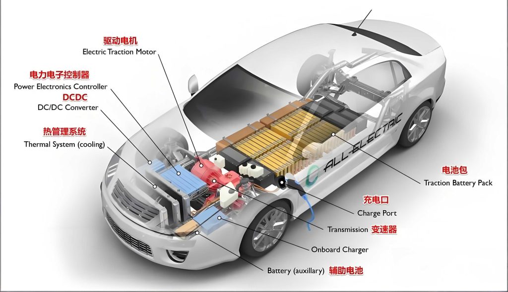
The battery system in a battery electric car is complex, consisting of multiple cells connected in series and parallel, along with a Battery Management System (BMS), sensors, and connectors. During operation, the internal state of lithium-ion batteries (LIBs) is not directly measurable, necessitating indirect methods for fault detection. Our approach focuses on online detection using real vehicle data to minimize computational cost and enable real-time monitoring. We select cell voltage as the primary fault feature due to its sensitivity to ISC faults and ease of measurement. The method involves data preprocessing, feature extraction using modified Empirical Mode Decomposition (EMD), Pearson Correlation Coefficient (PCC) analysis, sample entropy calculation, and improved Z-score for fault detection and localization.
Data for this study were sourced from a cloud-based big data platform compliant with national standards, which collects real-time operating data from battery electric cars. The data includes parameters such as current, cell voltages, state of charge (SOC), and temperature, recorded at intervals of 10 seconds. We processed data from multiple vehicles, including normal and faulty cases, to validate our method. The table below summarizes the vehicle data used:
| Vehicle ID | Collection Period | Number of Cells | Status | Fault Type |
|---|---|---|---|---|
| V1 | 2021-06-04 to 2021-08-25 | 97 | Normal | None |
| V2 | 2021-05-29 to 2021-09-14 | 95 | Faulty | Internal Short Circuit |
| V3 | 2021-05-31 to 2021-08-01 | 96 | Faulty | Voltage Inconsistency |
Data preprocessing is essential to ensure accuracy and reliability. We applied several steps: removal of duplicate records, elimination of outliers beyond the voltage range of 2.5V to 4.5V, and handling of missing values. For missing data, if fewer than three consecutive points were missing, interpolation using adjacent cell averages was performed; otherwise, the data segment was discarded. Additionally, we segmented data into charging and discharging processes based on current direction and SOC monotonicity, as faults may manifest differently in these phases. For a battery electric car, operational data can be noisy due to environmental factors, driving patterns, and sensor errors, so preprocessing enhances the robustness of subsequent analysis.
Feature extraction is centered on cell voltage, as it directly reflects cell behavior and is less delayed than temperature-based methods. In a series-connected battery pack, current is uniform, but voltages vary across cells, making voltage a suitable indicator for fault localization. However, raw voltage signals contain noise and trends that can obscure fault signatures. To address this, we employ a modified Empirical Mode Decomposition (EMD) method. EMD decomposes a signal into Intrinsic Mode Functions (IMFs) and a residual without requiring predefined basis functions, adapting to the signal’s time-scale characteristics. The standard EMD suffers from boundary effects and mode mixing, so we incorporate mirror symmetry extension and white noise assistance to improve decomposition accuracy. For a voltage signal $V(t)$ from a cell, the EMD process yields IMFs $c_j(t)$ and a residual $r(t)$ such that:
$$ V(t) = \sum_{j=1}^{n} c_j(t) + r(t) $$
where $n$ is the number of IMFs. Each IMF represents oscillatory components from high to low frequencies. We then compute the Pearson Correlation Coefficient (PCC) between each IMF (and the residual) and the original voltage to identify the component with the highest correlation. The PCC for two sequences $X$ and $Y$ is given by:
$$ \rho_{X,Y} = \frac{\sum_{i=1}^{N} (X_i – \bar{X})(Y_i – \bar{Y})}{\sqrt{\sum_{i=1}^{N} (X_i – \bar{X})^2 \sum_{i=1}^{N} (Y_i – \bar{Y})^2}} $$
where $\bar{X}$ and $\bar{Y}$ are means, and $N$ is the number of data points. The component with the highest absolute PCC value is selected as the new fault feature, as it retains the most relevant information about voltage variations while reducing noise.
For online detection, we use a sliding window (MW) approach to process data incrementally. The window size is set to 15 data points (equivalent to 150 seconds given the 10-second sampling interval), balancing sensitivity to faults and computational efficiency. As the window moves, we extract the new fault feature for each cell within the window and compute its sample entropy. Sample entropy (SampEn) quantifies the complexity or irregularity of a time series, with lower values indicating more regular patterns. For a time series $u(1), u(2), \ldots, u(N)$ of length $N$, SampEn is defined as follows. First, form vectors of dimension $m$: $x_m(i) = [u(i), u(i+1), \ldots, u(i+m-1)]$ for $i=1$ to $N-m+1$. Define the distance between vectors $x_m(i)$ and $x_m(j)$ as the maximum absolute difference between corresponding elements:
$$ d[x_m(i), x_m(j)] = \max_{k=0,\ldots,m-1} |u(i+k) – u(j+k)| $$
For a given tolerance $r$, count the number of vectors $j$ (with $j \neq i$) such that $d[x_m(i), x_m(j)] \leq r$, denoted as $B_i^m(r)$. Then, calculate:
$$ B^m(r) = \frac{1}{N-m} \sum_{i=1}^{N-m} B_i^m(r) $$
Similarly, for dimension $m+1$, count the number of matches $A_i^m(r)$ and compute:
$$ A^m(r) = \frac{1}{N-m} \sum_{i=1}^{N-m} A_i^m(r) $$
The sample entropy is then:
$$ \text{SampEn}(m, r) = -\ln \frac{A^m(r)}{B^m(r)} $$
In our implementation, we set $m=2$ and $r=0.2 \times \text{standard deviation of the data}$, as commonly recommended. Sample entropy values for each cell’s fault feature within the sliding window are computed to capture dynamic changes. To detect faults without setting fixed thresholds, we apply an improved Z-score method. For a set of sample entropy values $S_i$ for $i=1, 2, \ldots, n$ cells in a window, we calculate the mean $\bar{S}$ and standard deviation $\sigma$:
$$ \bar{S} = \frac{1}{n} \sum_{i=1}^{n} S_i $$
$$ \sigma = \sqrt{\frac{1}{n-1} \sum_{i=1}^{n} (S_i – \bar{S})^2} $$
The improved Z-score for cell $i$ is:
$$ Z_i = \frac{S_i – \bar{S}}{\sigma} $$
This Z-score normalizes the sample entropy values, with outliers indicating potential faults. A threshold of $|Z_i| > 3$ is typically used to flag anomalies, as values beyond three standard deviations are statistically significant. However, in practice, we monitor for sustained deviations across multiple windows to reduce false alarms. This method amplifies differences between normal and faulty cells, enabling precise fault localization without model dependency.
We validated our method using real vehicle data from the battery electric car platform. For normal vehicle V1, during a discharge process, all cells showed similar voltage profiles, and the computed sample entropy Z-scores remained below 3, indicating no faults. This aligns with the actual condition where no alerts were triggered. The results demonstrate that our method does not produce false positives under normal operation. For faulty vehicle V2, which experienced an ISC, cell #12 exhibited a voltage drop significantly larger than other cells over time. After applying EMD and PCC, the new fault feature retained this anomaly. The sample entropy Z-scores for cell #12 exceeded the threshold at the 216th sliding window, successfully detecting and localizing the fault. This early detection occurred while voltages were still within safe ranges, highlighting the method’s sensitivity.
To further illustrate the process, consider the following table summarizing key steps in our fault detection method for a battery electric car:
| Step | Description | Key Parameters | Output |
|---|---|---|---|
| Data Preprocessing | Clean and segment real vehicle data | Voltage range: 2.5V-4.5V; window for missing data | Processed time series for charging/discharging |
| Feature Extraction | Apply modified EMD to cell voltage | Number of IMFs; PCC threshold | New fault feature (highest correlation IMF) |
| Complexity Analysis | Compute sample entropy in sliding windows | $m=2$, $r=0.2 \times \text{std}$; window size=15 | Sample entropy values per cell per window |
| Fault Detection | Calculate improved Z-score for sample entropy | Mean and standard deviation of entropy values | Z-scores; fault flagged if $|Z| > 3$ |
| Localization | Identify cell with anomalous Z-score | Cell index; sustained deviations | Faulty cell ID and timing |
Our method was compared with two common fault detection approaches: threshold-based and PCC-based methods. The threshold method relies on preset voltage limits (e.g., overcharge or over-discharge thresholds) but fails to detect faults within safe ranges. The PCC-based method computes correlations between cell voltages but is sensitive to noise and cell inconsistencies, leading to reduced robustness. We tested these methods on vehicle V2 data. The threshold method did not trigger any alarms since voltages remained within bounds, while the PCC method showed high correlations across all cells, missing the fault. In contrast, our method successfully detected the ISC fault. The comparison is summarized below:
| Method | Accuracy | Model Required | Robustness | Online Capability |
|---|---|---|---|---|
| Threshold-Based | Low | No | Poor | Yes |
| PCC-Based | Moderate | No | Moderate | Yes |
| Our Method | High | No | Strong | Yes |
Robustness analysis was performed using vehicle V3, which had voltage inconsistency but no ISC fault. Without preprocessing to handle cell consistency, the Z-scores occasionally spiked, causing false alarms. However, after applying boxplot analysis to identify and remove outliers from inconsistent cells, the Z-scores remained below the threshold, demonstrating the necessity of data preprocessing for reliable fault diagnosis in battery electric cars. The boxplot method identifies cells with voltages outside the interquartile range (IQR) as anomalies, where IQR = Q3 – Q1, and bounds are set at Q1 – 1.5*IQR and Q3 + 1.5*IQR. This step ensures that inherent cell variations do not misinterpret as faults.
The advantages of our method are multifold for battery electric car applications. First, it is data-driven, eliminating the need for complex battery models that are difficult to derive for real-world conditions. Second, it operates online with low computational cost, as the sliding window processes only recent data, reducing memory requirements and enabling real-time implementation on embedded systems like BMS. Third, it avoids threshold setting by using statistical Z-scores, making it adaptable to different vehicle models and battery types. Fourth, it enhances sensitivity to early-stage faults like ISC, which are critical for preventing thermal runaway. The integration of EMD and sample entropy captures nonlinear dynamics in voltage signals, which are often indicative of faults.
To delve deeper into the mathematical foundation, let’s consider the sample entropy calculation in more detail. For a time series representing the new fault feature $F(t)$ within a sliding window of length $L=15$, we have $F(1), F(2), \ldots, F(L)$. The sample entropy parameters $m$ and $r$ are chosen based on typical values for physiological and engineering signals. The tolerance $r$ is proportional to the data’s standard deviation to ensure consistency across different scales. The sample entropy formula can be expressed algorithmically as:
- Set $m=2$, $r=0.2 \times \sigma_F$, where $\sigma_F$ is the standard deviation of $F$.
- Form vectors $x_m(i) = [F(i), F(i+1)]$ for $i=1$ to $L-m$.
- Compute distances $d[i,j] = \max(|F(i)-F(j)|, |F(i+1)-F(j+1)|)$.
- Count matches where $d[i,j] \leq r$ for $j \neq i$ to get $B_i$ and $A_i$ for $m+1=3$.
- Average to find $B^m(r)$ and $A^m(r)$, then compute SampEn.
This process is repeated for each cell in every sliding window. The computational complexity is $O(L^2)$ per window, but since $L$ is small, it is feasible for online use. The improved Z-score then standardizes these entropy values. For a battery electric car with $n$ cells, the overall complexity per window is $O(n \cdot L^2)$, which is manageable for typical BMS hardware.
In terms of practical implementation, the method can be integrated into the BMS of a battery electric car to provide continuous monitoring. The BMS already collects voltage data, so additional processing can be added via software updates. The algorithm flow is as follows: acquire real-time cell voltages, preprocess to remove noise and outliers, decompose using EMD, select the highest-correlation component, compute sample entropy in a sliding window, calculate Z-scores, and trigger alerts if anomalies persist. This enables proactive maintenance and enhances safety for battery electric car users.
We also explored the impact of window size on detection performance. A smaller window increases sensitivity to rapid changes but may raise false alarms due to noise, while a larger window smoothens signals but could delay detection. Through empirical testing on real vehicle data, we found that a window size of 15 samples (150 seconds) offers a good balance. This corresponds to approximately 2.5 minutes of data, capturing enough dynamics without excessive lag. The table below shows how detection time varies with window size for vehicle V2’s ISC fault:
| Window Size (samples) | Detection Time (sliding window index) | False Alarm Rate | Remarks |
|---|---|---|---|
| 10 | 210 | High | Early but noisy |
| 15 | 216 | Low | Optimal balance |
| 20 | 225 | Low | Delayed detection |
Furthermore, the method’s robustness to different driving conditions was assessed. Battery electric cars operate in diverse environments—urban stop-and-go traffic, highway cruising, and varying temperatures—all affecting battery behavior. Our data preprocessing includes filtering for extreme values, but the EMD and sample entropy steps inherently handle non-stationary signals. EMD adapts to local time scales, making it suitable for the fluctuating loads typical in battery electric car usage. Sample entropy, as a nonlinear measure, captures complexity changes even when voltage trends are non-uniform.
For future work, we plan to extend this method to other fault types in battery electric cars, such as external short circuits or connection failures, by incorporating additional features like current and temperature. Fusion of multiple data sources could improve diagnosis accuracy. Additionally, machine learning techniques could be integrated to adaptive threshold tuning based on historical data. However, the current approach stands as a lightweight, effective solution for online ISC detection.
In conclusion, our proposed fault detection method for battery electric car systems demonstrates high efficacy using real vehicle data. It leverages modified EMD, PCC, sample entropy, and improved Z-scores to achieve online detection of internal short circuits without requiring battery models or fixed thresholds. The method is computationally efficient, robust to noise, and adaptable to various vehicle types. Validation on real-world data from battery electric cars confirms its ability to detect faults early while minimizing false alarms. This contributes to the safety and reliability of battery electric cars, supporting the broader adoption of electric mobility. As the industry evolves, such data-driven approaches will be crucial for advancing battery management systems and ensuring user confidence in battery electric car technology.