
In this paper, I present a comprehensive study on the design, calibration, and error optimization of a Hall element elliptical array current sensor specifically developed for high-current measurement in EV battery pack systems. The growing demand for lightweight, compact, and cost-effective current sensing solutions in new energy vehicles has motivated this work. Conventional current transducers based on magnetic cores or shunt resistors face limitations in terms of size, weight, and accuracy under harsh automotive conditions. To address these challenges, I propose a Hall array architecture without a magnetic core, which measures the magnetic field around a rectangular busbar and reconstructs the current via Ampere’s circuital law. The elliptical arrangement reduces the installation footprint while maintaining high fidelity of the field integration. I further design a full temperature-domain calibration algorithm to compensate for initial offset and sensitivity drift, and develop a Grey Wolf Optimizer–Backpropagation neural network model to estimate conductor eccentricity and tilt parameters, thereby minimizing measurement errors. Extensive simulations and experiments confirm that the proposed sensor achieves a measurement accuracy better than 3‰ across the temperature range from -40 °C to 125 °C, and significantly reduces eccentricity and tilt errors. This work provides an effective solution for accurate and compact current measurement in EV battery pack applications.
1. Introduction
With the intensifying global energy crisis and the urgent need for environmental protection, the transition toward low-carbon transportation has accelerated dramatically. New energy vehicles, particularly battery electric vehicles, have become the mainstream of future mobility. In 2023, the production and sales of new energy vehicles in China reached approximately 9.5 million units, and the export value of new energy vehicles, lithium batteries, and photovoltaic cells exceeded one trillion yuan for the first time. It is expected that by 2030, the number of new energy vehicles on the road will reach around 100 million, representing a market share of more than 70%.
Lithium-ion power batteries are widely adopted in new energy vehicles due to their high energy density, high power density, long cycle life, and zero memory effect. However, safety concerns such as thermal runaway and fire accidents remain critical issues. Statistics indicate that about 90% of new energy vehicle accidents are related to power battery problems. The battery management system (BMS) plays an essential role in monitoring the state of the battery pack, including voltage, current, temperature, and insulation resistance. Among these parameters, current is one of the most important variables for state-of-charge estimation, state-of-health assessment, and fault diagnosis. Therefore, a high-precision, compact, and reliable current sensor is crucial for the safety and performance of EV battery pack systems.
Traditional current sensors used in BMS include shunt resistors, fluxgate sensors, and closed-loop Hall sensors. Shunt resistors are contact-based and introduce power losses and galvanic coupling, increasing the complexity of electrical isolation. Fluxgate sensors offer high accuracy but suffer from magnetic saturation, hysteresis, and large volume. Conventional Hall sensors require a magnetic core to concentrate the field, which increases weight and footprint. Moreover, the demand for lightweight and integrated designs in modern EV battery pack systems makes these conventional solutions less attractive.
Hall array current sensors, which eliminate the magnetic core by arranging multiple Hall elements around the conductor, have emerged as a promising alternative. This type of sensor reconstructs the current by numerically integrating the tangential magnetic field along a closed loop around the busbar. Compared with core-based sensors, the array sensor is immune to magnetic saturation and hysteresis, and offers advantages in size, weight, and cost. Nevertheless, the accuracy of Hall array sensors is affected by the number and arrangement of Hall elements, initial manufacturing tolerances, temperature drift, conductor eccentricity, and conductor tilt. These issues must be addressed to meet the stringent requirements for EV battery pack current measurement.
The objective of this research is to develop a Hall element elliptical array current sensor tailored for rectangular busbars in EV battery pack systems. The elliptical shape allows the sensor to fit the elongated cross-section of the rectangular conductor, significantly reducing the installation area compared with a circular array and providing a smoother magnetic field gradient than a rectangular array. I systematically investigate the array parameter design, hardware implementation, full-range temperature calibration, and advanced error compensation using a hybrid GWO-BP neural network.
The remainder of this paper is organized as follows: Section 2 reviews the fundamentals of magnetic sensing and Hall effect. Section 3 presents the design of the elliptical Hall array, including the generation method, parameter optimization, and hardware implementation. Section 4 analyzes the error sources and proposes the calibration and optimization algorithms. Section 5 describes the simulation environment, experimental setup, and performance evaluation. Finally, Section 6 concludes the paper and discusses future work.
2. Fundamentals of Magnetic Sensors
2.1 Magnetic Fluxgate and Hall Effect
Magnetic sensors convert magnetic field information into electrical signals. Two common principles are the fluxgate effect and the Hall effect. The fluxgate effect relies on the nonlinear relationship between the magnetic permeability of soft magnetic materials and the magnetic induction intensity. When the core approaches saturation, the permeability changes dramatically, allowing the detection of weak magnetic fields. Fluxgate sensors have high resolution, typically reaching 1 pT, but they require complex excitation circuits and are difficult to miniaturize.
The Hall effect was discovered by Edwin Hall in 1879. When a current-carrying conductor is placed in a perpendicular magnetic field, the charge carriers experience a Lorentz force, leading to a transverse voltage known as the Hall voltage. This voltage is proportional to the magnetic flux density perpendicular to the current direction. For a semiconductor plate of thickness \(d\), the Hall voltage can be expressed as:
$$ V_H = \frac{IB}{nqd} $$
where \(I\) is the current through the Hall plate, \(B\) is the magnetic flux density, \(n\) is the charge carrier concentration, \(q\) is the elementary charge, and \(d\) is the thickness of the plate. The sensitivity coefficient \(K_H = 1/(nqd)\) is usually defined, so that \(V_H = K_H I B\). Hall elements are widely used because of their good linearity, low cost, small size, and ease of integration. However, their temperature dependence and offset voltage must be compensated.
2.2 Open-Loop and Closed-Loop Hall Current Sensors
Open-loop Hall current sensors consist of a magnetic core with an air gap, a Hall element placed in the gap, and signal conditioning circuits. The core concentrates the magnetic field generated by the primary current. The Hall voltage is proportional to the magnetic field in the gap, which, according to Ampere’s law, is proportional to the primary current when the core is not saturated. The open-loop configuration is simple and low-cost, but its accuracy is limited by temperature drift and core nonlinearity.
Closed-loop Hall current sensors add a secondary winding and an operational amplifier to generate a compensating current that cancels the primary field. The sensor works in a null-balance mode, which greatly improves linearity and reduces temperature effects. However, the compensation coil increases the complexity and power consumption, and the magnetic core still limits the bandwidth and size.
To overcome the drawbacks of magnetic cores, the array-based Hall current sensor has been developed. In this concept, multiple Hall elements are placed around the conductor without any magnetic core. The current is calculated by integrating the measured tangential magnetic field along a closed path:
$$ I = \oint \mathbf{H} \cdot d\mathbf{l} $$
where \(\mathbf{H}\) is the magnetic field intensity and \(d\mathbf{l}\) is the infinitesimal path element. With only \(N\) discrete Hall elements, the integral is approximated by a summation:
$$ I_{\text{calc}} = \sum_{i=1}^{N} H_{\text{MFS},i} \, \Delta s_i $$
where \(H_{\text{MFS},i}\) is the measured field component along the sensor’s sensitive direction at the \(i\)-th Hall element, and \(\Delta s_i\) is the length of the corresponding curve segment. The accuracy of this approximation depends on the number of Hall elements and their arrangement.
2.3 Array Configurations and the Elliptical Array
Several array geometries have been studied, including circular, rectangular, linear, and elliptical arrays. Circular arrays are natural for circular conductors, but they are inefficient for rectangular cross-sections because the large radius increases the distance between the sensors and the conductor, reducing the signal-to-noise ratio. Rectangular arrays match the shape of the busbar but suffer from steep magnetic field gradients near the corners, leading to integration errors. The elliptical array offers a compromise: it wraps closer to the rectangular contour while maintaining a smooth curvature, resulting in a smaller area and a more uniform magnetic field distribution along the array.
In this work, I focus on the elliptical Hall array for measuring rectangular conductors inside an EV battery pack. A typical rectangular busbar used in EV battery pack has dimensions of 20 mm × 4 mm. The required measurement range is up to ±1500 A, with an accuracy target of 3‰ or better over a wide temperature range.
3. Design of the Hall Array Current Sensor
3.1 Generation of the Elliptical Array
Two methods are commonly used to distribute Hall elements on an ellipse: the projection method and the uniform curve segment length (UCSL) method. The projection method projects equally spaced points from a circle onto the ellipse, which results in non-uniform arc lengths. In contrast, the UCSL method divides the ellipse perimeter into equal arc segments, ensuring that each Hall element corresponds to the same path length contribution. I adopt the UCSL method because it yields lower current reconstruction errors for the same number of Hall elements.
For an ellipse with semi-major axis \(a\) and semi-minor axis \(b\), the perimeter is approximated numerically by sampling points. Let the ellipse be discretized into \(K\) points (e.g., \(K \ge 5\times 10^6\)). The coordinates of the \(k\)-th point are:
$$ E_k = \left( a \cos\frac{360^\circ \cdot k}{K}, \ b \sin\frac{360^\circ \cdot k}{K} \right) $$
For a chosen number of Hall elements \(N\), the arc length of each segment is \(\Delta s = s(K)/N\), where \(s(K)\) is the total perimeter. An initial offset parameter \(s_{0,r}\) is introduced to improve robustness. The position of the \(i\)-th Hall element \(P_{i-1}\) is found by locating the point where the cumulative arc length equals \(s_i = s_0 + i\Delta s\). The tangent vector at that point defines the sensitive direction.
To compare the two generation methods, I computed the theoretical current error as a function of the number of Hall elements for a fixed ellipse with \(a=30\) mm. The results show that the UCSL method consistently outperforms the projection method. Therefore, I use the UCSL method throughout the design.
3.2 Parameter Optimization
The key parameters are the number of Hall elements \(N\) and the aspect ratio \(AR = b/a\). The current error \(\varepsilon\) is calculated as:
$$ \varepsilon = \frac{I_{\text{calc}} – I}{I} \times 100\% $$
where \(I\) is the actual current and \(I_{\text{calc}}\) is the reconstructed value. Using MATLAB simulations, I evaluated the current error for different \(N\) and \(AR\) values. Figure 3-3 in the original paper (not reproduced here) shows that the error decreases as \(N\) increases, but the improvement saturates for \(N>7\). Considering cost and complexity, I restrict the study to \(N=6\) and \(N=7\).
The relationship between aspect ratio and current error, shown in Figure 3-4 of the original paper, indicates that for the circular array (\(AR=1\)), the error is zero for ideal positioning. However, the circle requires a large installation area. For elliptical arrays, certain combinations of \(N\) and \(AR\) yield theoretically zero error. For example, \(N=6, AR=0.33\) and \(N=7, AR=0.31\) produce good performance. Table 3-1 summarizes the Hall element positions and sensitive directions for four selected configurations: (i) \(N=6, AR=0.33\); (ii) \(N=7, AR=0.31\); (iii) \(N=6, AR=1\); (iv) \(N=7, AR=1\). These are used for comparison in the subsequent analysis.
| Configuration | \(s_{0,r}\) | Hall element positions \(P_{i-1}\) | Sensitive directions \(t_{i-1}\) |
|---|---|---|---|
| \(N=6, AR=0.33\) | 0.0417 | (26.94, 4.40), (5.57, 9.83), (-16.59, 8.33), (-26.94, -4.40), (-5.56, -9.83), (16.59, -8.33) | (-0.827, 0.563), (-0.998, 0.063), (-0.976, -0.216), (0.827, -0.563), (0.998, -0.063), (0.976, 0.216) |
| \(N=7, AR=0.31\) | 0.0179 | (29.18, 2.17), (11.77, 8.55), (-7.07, 9.04), (-25.41, 4.95), (-21.01, -6.64), (-2.36, -9.27), (16.43, -7.78) | (-0.611, 0.791), (-0.991, 0.131), (-0.997, -0.075), (-0.897, -0.443), (0.957, -0.291), (1.000, -0.024), (0.980, 0.199) |
For a rectangular busbar of 20 mm × 4 mm, I set the semi-major axis \(a = 30\) mm to provide sufficient clearance and to accommodate the insulating layers and the printed circuit board. The allowable eccentricity ranges are listed in Table 4-1 of the original paper. The elliptical array with \(AR=0.33\) allows X-direction eccentricity up to ±10.5 mm, while the Y-direction allowable eccentricity is only ±2.1 mm due to the small semi-minor axis. In practice, Y-direction displacement is limited by the narrow dimension of the busbar, so the ellipse remains a viable solution.
3.3 Hall Element Selection
The selection of Hall elements is critical for the overall performance. I considered sensitivity, saturation field, temperature coefficient, and nonlinearity. For the single-axis sensors in the elliptical array, the AKM EQ-730L Hall element was selected. Its key parameters are listed in Table 3-2.
| Parameter | Symbol | Min | Typical | Max | Unit |
|---|---|---|---|---|---|
| Supply voltage | \(V_{cc}\) | 3.0 | 5.0 | 5.5 | V |
| Supply current | \(I_{cc}\) | -12 | – | 12 | mA |
| Output voltage | \(V_{out}\) | 10 | – | 90 | % \(V_{cc}\) |
| Sensitivity | \(V_h\) | 110 | 130 | 150 | mV/mT |
| Temperature range | \(T\) | -40 | 25 | 125 | °C |
For the three-axis measurements needed to estimate the conductor state (especially tilt), I selected the Infineon TLV493DA1B6 three-axis Hall sensor. This sensor provides X, Y, and Z magnetic field components with a 12-bit resolution. Table 3-4 lists its main characteristics.
| Parameter | Symbol | Min | Typical | Max | Unit |
|---|---|---|---|---|---|
| Supply voltage | \(V_{DD}\) | 2.8 | 3.3 | 3.5 | V |
| Sensitivity | \(V_h\) | – | 10.2 | – | LSB12/mT |
| Average operating current | \(I_{DD(op)}\) | – | 3.7 | – | mA |
| Temperature range | \(T\) | -40 | – | 125 | °C |
3.4 Hardware Circuit Design
The current sensor hardware includes the Hall element array, an analog conditioning circuit, a microcontroller, a power management unit, and a CAN communication interface. The sensor is powered from a 12 V DC source, which is converted to 5 V by an E1205SY DC-DC module. The 5 V supply powers the Hall elements and the operational amplifiers. A TLV1117 low-dropout regulator further provides 3.3 V for the STM32F103C8T6 microcontroller.
The analog signals from six EQ-730L Hall elements are first buffered by voltage followers. A summing amplifier combines the six voltages to produce a total signal proportional to the line integral of the magnetic field. The total voltage and the individual Hall voltages are digitized by the microcontroller’s 12-bit ADC. The microcontroller computes the current and transmits the result through a TJA1050 CAN transceiver to the upper computer. The power supply and interface circuits are shown in Figures 3-9 through 3-12 of the original paper, which I have implemented as printed circuit board modules.
4. Error Analysis and Optimization
4.1 Initial Error and Full Temperature-Domain Calibration
Initial errors arise from the offset and gain drift of the Hall elements and the analog circuit. To reduce these errors, I designed a calibration algorithm that operates over the full temperature range. The calibration process is performed offline in a temperature chamber and the resulting compensation coefficients are stored in the microcontroller’s memory.
At room temperature (25 °C), I measure the sensor’s output for different current values from -1500 A to +1500 A. The raw digital signal \(ADC_{\text{diff}}\) is the difference between the high-order and low-order 16-bit readings. The sampled voltage is:
$$ V_{\text{ADC}} = \frac{ADC_{\text{diff}} \cdot V_{\min}}{K \cdot A} $$
where \(V_{\min}=0.001\) V is the minimum resolvable voltage, \(K=128\) is the number of samples, and \(A\) is the gain factor. For currents from 0 to 90 A, \(A=100\); from 91 to 870 A, \(A=10\); and from 871 to 1500 A, \(A=5\). The measured current is:
$$ I_{\text{output}} = \frac{V_{\text{ADC}}}{R} $$
with \(R=0.47\,\Omega\). The current deviation is \(\Delta I = I_{\text{output}}-I_{\text{input}}\). I then perform a least-squares linear fit for each current segment:
$$ \Delta I_{\text{fit}} = k_i I_{\text{output}} + b_i $$
where \(i\) indexes the segment and direction. The calibration coefficient \(k_i\) and \(b_i\) are determined by minimizing the squared error. The compensated current is obtained by subtracting the fitted deviation:
$$ I_{\text{mea}} = I_{\text{output}} – \Delta I_{\text{fit}} $$
The residual relative error is:
$$ \Delta_{\text{rel}} = \frac{I_{\text{mea}} – I_{\text{input}}}{I_{\text{input}}} \times 1000‰ $$
Additionally, I compared the linear fit with a quadratic fit. The linear fit provides better overall residual performance and is simpler to implement. Therefore, I adopt the linear calibration model.
To account for temperature drift, I perform the calibration at three temperatures: -40 °C, 25 °C, and 125 °C. For each temperature \(T\), I obtain the slope \(k_T\) and intercept \(b_T\) from the linear fit. The temperature drift coefficient \(k_{\text{drift}}\) is computed from the slope difference between adjacent temperatures divided by the temperature difference. Specifically, the low-temperature drift coefficient is:
$$ k_{\text{low}} = \frac{k_{-40} – k_{25}}{65} $$
and the high-temperature drift coefficient is:
$$ k_{\text{high}} = \frac{k_{125} – k_{25}}{100} $$
The unit temperature drift coefficient is the average:
$$ \bar{k} = \frac{k_{\text{low}} + k_{\text{high}}}{2} $$
The final temperature-compensated deviation is computed as:
$$ \Delta I_{\text{fit,temp}} = (k_i + \bar{k} \cdot T) \, I_{\text{output}} + b_i $$
and the compensated current is \(I_{\text{mea,temp}} = I_{\text{output}} – \Delta I_{\text{fit,temp}}\). This full temperature-domain calibration reduces the initial error to below 3‰ across the entire temperature range.
4.2 Current Inversion Model with Eccentricity and Tilt
When the conductor is eccentrically positioned or tilted relative to the array plane, the magnetic field distribution changes, causing reconstruction errors. To analyze these errors, I developed a three-dimensional magnetic field model and an inversion formula. The geometry is shown in Figure 4-2 of the original paper: the ellipse lies in the XOY plane, with the conductor axis intersecting XOY at point \(Q(x_0, y_0, 0)\). The conductor tilt is described by two angles: \(\alpha\) (angle between the conductor axis and the positive Z-axis) and \(\beta\) (angle between the projection of the conductor axis on the XOY plane and the positive X-axis). Thus, the conductor direction vector is:
$$ \mathbf{l} = (m, n, p) = (\sin\alpha \cos\beta,\ \sin\alpha \sin\beta,\ \cos\alpha) $$
For a point \(P(a,b,0)\) on the ellipse, the vector from \(Q\) to \(P\) is \(\overrightarrow{QP}\). The perpendicular distance from the conductor to point P is:
$$ \rho = \|\mathbf{l} \times \overrightarrow{QP}\| $$
The magnetic field due to an infinitely long straight conductor is:
$$ \mathbf{H} = \frac{I}{2\pi\rho} \, \mathbf{e}_l \times \mathbf{e}_r $$
where \(\mathbf{e}_l\) is the unit vector along the conductor, and \(\mathbf{e}_r\) is the unit vector from \(Q\) to \(P\). For a rectangular conductor of cross-sectional area \(A\), the magnetic field components at point \((a,b,0)\) are obtained by integrating the current density over the cross-section \(S\):
$$ H_x = \frac{I}{2\pi A} \int_S \frac{p(b-y)}{p^2(a-x)^2 + p^2(b-y)^2 + [m(a-x)+n(b-y)]^2} \, dxdy $$
$$ H_y = \frac{I}{2\pi A} \int_S \frac{p(a-x)}{p^2(a-x)^2 + p^2(b-y)^2 + [m(a-x)+n(b-y)]^2} \, dxdy $$
$$ H_z = \frac{I}{2\pi A} \int_S \frac{m(a-x)+n(b-y)}{p^2(a-x)^2 + p^2(b-y)^2 + [m(a-x)+n(b-y)]^2} \, dxdy $$
The integration region \(S\) is the projection of the actual conductor cross-section onto the XOY plane. When the conductor is tilted, the projection changes shape and size. When the conductor is eccentrically shifted, the projection shifts by \(X_p\) and \(Y_p\). The boundaries of the integration region can be derived from the conductor dimensions and the tilt parameters. I developed a computation routine that constructs the integration region equation for any given \((X_p,Y_p,m,n,p)\).
For the ideal vertical conductor, \((m,n,p)=(1,1,0)\) (with the appropriate sign for z direction), and the 3D equations reduce to the standard 2D formulas. At each Hall element, the field along its sensitive direction is the dot product of the local field vector with the sensitive axis unit vector. The current is then computed by summing the products of these tangential field components with the corresponding arc lengths:
$$ I_{\text{calc}} = \sum_{i=0}^{5} H_{i} \, \Delta s $$
where \(\Delta s\) is the same for all segments under the UCSL method.
4.3 Eccentricity and Tilt Error Analysis
Using the inversion model, I analyzed the theoretical current error due to purely X-direction eccentricity and purely Y-direction eccentricity for four array configurations. The allowable eccentricity ranges are given in Table 4-1.
| Configuration | -X limit (mm) | +X limit (mm) | -Y limit (mm) | +Y limit (mm) |
|---|---|---|---|---|
| \(N=6, AR=0.33\) | -10.5 | 10.5 | -2.1 | 2.1 |
| \(N=7, AR=0.31\) | -10.7 | 10.7 | -2.0 | 2.0 |
| \(N=6, AR=1\) | -14.9 | 14.9 | -20.9 | 20.9 |
| \(N=7, AR=1\) | -14.9 | 14.9 | -20.9 | 20.9 |
Figure 4-4 of the original paper demonstrates that the current error increases with increasing eccentricity. For X-direction eccentricity up to about 10 mm, the error for the elliptical array can reach 4.18%, which exceeds the acceptable ±1% tolerance. For Y-direction eccentricity up to 2.4 mm, the error reaches about 0.94%. These results indicate the necessity of an error compensation algorithm. Although the circular array allows larger X and Y displacements, its larger footprint (2827 mm²) compared with the elliptical array (908.5 mm²) makes it less suitable for compact EV battery pack integration. The weight of the elliptical array sensor is 11.9 g versus 15.5 g for the circular array and 69.5 g for a fluxgate sensor. This reduces the installation footprint by 72.4% and weight by 82.9% compared with the fluxgate solution.
4.4 GWO-BP Neural Network for Conductor State Estimation
To compensate for eccentricity and tilt errors, I need to accurately estimate the conductor state parameters \((X_p,Y_p,m,n,p)\). Since these parameters are nonlinearly related to the measured magnetic field components at the Hall positions, a neural network approach is suitable. I use a BP neural network with one hidden layer, but the standard BP algorithm is prone to local optima and slow convergence. To overcome this, I employ the Grey Wolf Optimizer (GWO) to optimize the initial weights and thresholds of the BP network.
The GWO algorithm mimics the hunting behavior of grey wolves. The population is divided into four levels: \(\alpha\), \(\beta\), \(\delta\), and \(\omega\). The positions of the wolves are updated according to the following equations:
$$ \mathbf{D} = |\mathbf{C} \mathbf{X}_p(t) – \mathbf{X}(t)| $$
$$ \mathbf{X}(t+1) = \mathbf{X}_p(t) – \mathbf{A} \cdot \mathbf{D} $$
where \(\mathbf{A}\) and \(\mathbf{C}\) are coefficient vectors:
$$ \mathbf{A} = 2a\mathbf{r}_1 – a, \quad \mathbf{C} = 2\mathbf{r}_2 $$
Here \(\mathbf{r}_1, \mathbf{r}_2\) are random vectors in [0,1], and \(a\) decreases linearly from 2 to 0 over the iterations. The position of \(\omega\) wolves is updated based on the top three solutions \(\mathbf{X}_\alpha, \mathbf{X}_\beta, \mathbf{X}_\delta\):
$$ \mathbf{X}_\omega(t+1) = \frac{\mathbf{X}_\alpha + \mathbf{X}_\beta + \mathbf{X}_\delta}{3} $$
In the GWO-BP model, the weight vector of the BP network is encoded as the position of a grey wolf. The fitness function is the mean squared error between the predicted and actual conductor state parameters. The GWO searches for the optimal weight vector that minimizes the fitness.
The network structure is configured as follows: the input layer has 18 nodes (6 Hall elements × 3 magnetic field components: Bx, By, Bz). The hidden layer has 12 nodes (determined by trial). The output layer has 5 nodes, corresponding to \((X_p, Y_p, m, n, p)\). The GWO parameters are set to a population size of 20 and a maximum of 50 iterations. The algorithm flowchart is described in Figure 4-8 of the original paper.
After the conductor state parameters are estimated, the integration region is reconstructed, and the magnetic field components are recomputed using the 3D equations. This yields a corrected current value with significantly reduced eccentricity and tilt errors.
5. Testing and Performance Evaluation
5.1 Test Platform
I built a test platform comprising an industrial PC (ADVANTECH IPC-610-L), a high-power programmable DC source (AMETEK Sorensen SGX) capable of generating currents up to 1500 A, a current commutation module based on an Arduino Nano, a KEITHLEY DAQ6510 data acquisition system, a TONGHUI TH6313 programmable DC supply for the sensor’s power, and a BOYI B-TH-120B temperature chamber for temperature-controlled tests. The upper computer runs a LabVIEW-based software platform that manages the test flow, collects data, and stores the results. The test platform diagram and system flow are described in Figures 5-7 and 5-9.
The software platform allows multiple current points and multiple temperature points to be programmed. The test sequence automatically steps through the specified currents and temperatures, waiting for the chamber to stabilize before recording data.
5.2 Finite Element Simulation
I performed finite element simulations using COMSOL Multiphysics to verify the magnetic field distribution around a rectangular conductor and to generate training data for the neural network. The simulated conductor was a 20 mm × 4 mm copper busbar with a conductivity of \(5.998 \times 10^7\) S/m. The surrounding air domain was modeled as air with zero conductivity. The simulation mesh was adaptively refined. The resulting magnetic flux density distribution confirmed that the field contours are elliptical, which supports the use of an elliptical array. The simulation data were exported to MATLAB to create the dataset for the GWO-BP model.
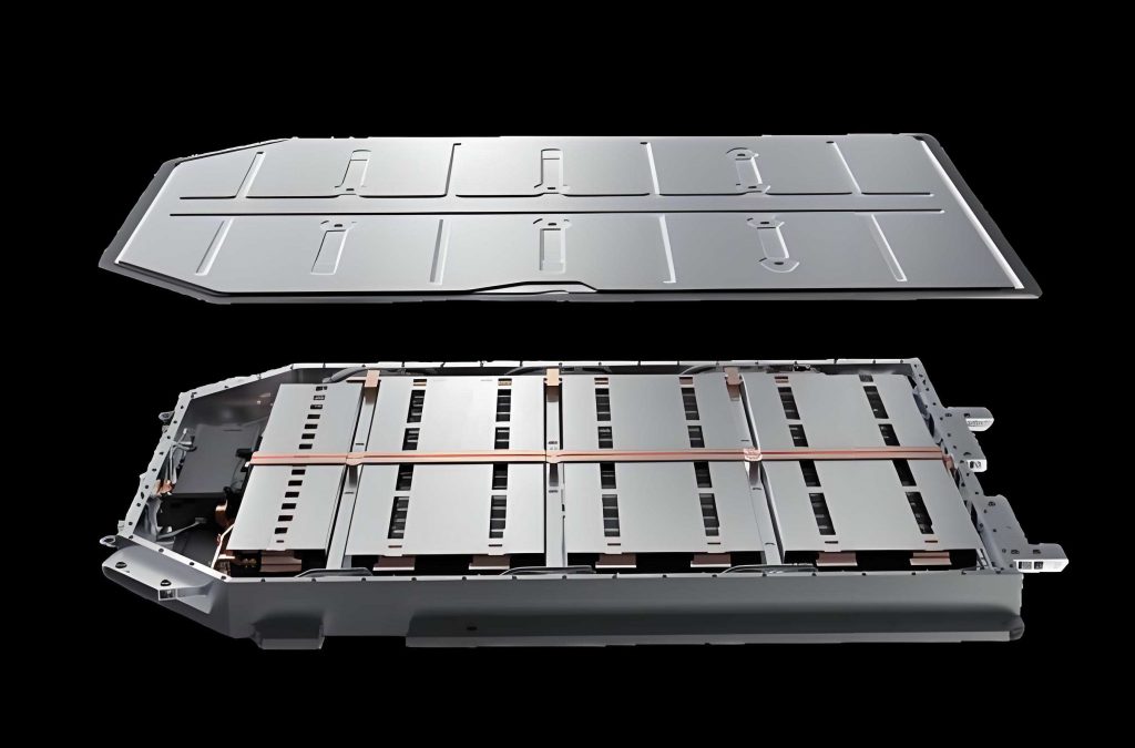
Figure 5-11 in the original paper shows the magnetic flux density distribution. I inserted the relevant image from the shared resource to illustrate the magnetic field pattern. The image is reproduced below.
5.3 Performance of the Conductor State Estimation Model
I evaluated the GWO-BP model using three metrics: mean absolute error (MAE), mean squared error (MSE), and mean absolute percentage error (MAPE). The metrics are defined as:
$$ \text{MAE} = \frac{1}{n}\sum_{i=1}^{n}\left| y_i – \hat{y}_i \right| $$
$$ \text{MSE} = \frac{1}{n}\sum_{i=1}^{n}\left( y_i – \hat{y}_i \right)^2 $$
$$ \text{MAPE} = \frac{1}{n}\sum_{i=1}^{n}\left| \frac{y_i – \hat{y}_i}{y_i} \right| \times 100\% $$
Table 5-2 compares the BP and GWO-BP models for estimating each conductor state parameter.
| Parameter | Algorithm | MAE | MSE | MAPE |
|---|---|---|---|---|
| \(X_p\) | BP | 0.2272 | 0.0771 | 0.8419% |
| GWO-BP | 0.0498 | 0.0041 | 1.0411% | |
| \(Y_p\) | BP | 0.0619 | 0.0043 | 5.2646% |
| GWO-BP | 0.0146 | 0.0004 | 1.0621% | |
| \(m\) | BP | 0.0124 | 0.0003 | 10.3490% |
| GWO-BP | 0.0037 | 0.0001 | 2.8585% | |
| \(n\) | BP | 0.0071 | 0.0002 | 3.9567% |
| GWO-BP | 0.0028 | 0.0001 | 0.8626% | |
| \(p\) | BP | 0.0143 | 0.0005 | 2.2479% |
| GWO-BP | 0.0029 | 0.0001 | 0.4173% |
The results indicate that the GWO-BP model significantly reduces MAE and MSE compared with the standard BP model, although the MAPE for \(X_p\) is slightly higher. The GWO-BP model provides more stable and accurate estimates, leading to better compensation of the current errors. The overall performance demonstrates the advantage of the GWO-BP approach in handling complex multidimensional regression tasks.
5.4 Full Temperature-Domain Calibration Results
I performed the calibration experiments inside the temperature chamber at -40 °C, 25 °C, and 125 °C. The current was swept from -1500 A to +1500 A in steps. The measured current deviation before and after calibration is shown in Figures 5-15 through 5-20 of the original paper. For clarity, I summarize the calibration equations in Table 5-3.
| Temperature | Segment | Direction | Slope | Intercept |
|---|---|---|---|---|
| -40 °C | Small current | Positive | \(k_0=-0.00349\) | \(b_0=0.03591\) |
| Negative | \(k_1=-0.00369\) | \(b_1=-0.04803\) | ||
| Medium current | Positive | \(k_2=-0.00380\) | \(b_2=-0.23163\) | |
| Negative | \(k_3=-0.00392\) | \(b_3=0.22826\) | ||
| Large current | Positive | \(k_4=-0.00272\) | \(b_4=-0.99071\) | |
| Negative | \(k_5=-0.00293\) | \(b_5=0.91182\) | ||
| 25 °C | Small current | Positive | \(k_0=-0.00505\) | \(b_0=0.04657\) |
| Negative | \(k_1=-0.00508\) | \(b_1=-0.04342\) | ||
| Medium current | Positive | \(k_2=-0.00367\) | \(b_2=0.06019\) | |
| Negative | \(k_3=-0.00395\) | \(b_3=-0.10566\) | ||
| Large current | Positive | \(k_4=-0.00284\) | \(b_4=-1.12625\) | |
| Negative | \(k_5=-0.00316\) | \(b_5=1.12059\) | ||
| 125 °C | Small current | Positive | \(k_0=0.00369\) | \(b_0=-0.07629\) |
| Negative | \(k_1=-0.00386\) | \(b_1=-0.21222\) | ||
| Medium current | Positive | \(k_2=0.00421\) | \(b_2=-0.65411\) | |
| Negative | \(k_3=0.00387\) | \(b_3=0.31021\) | ||
| Large current | Positive | \(k_4=0.00618\) | \(b_4=-2.03248\) | |
| Negative | \(k_5=0.00564\) | \(b_5=1.52958\) |
After calibration, the relative current error was reduced to less than 3‰ at all temperatures. Specifically, the room-temperature error was reduced by 85.58%, the low-temperature error by 62.59%, and the high-temperature error by 42.99%. These results confirm the effectiveness of the full temperature-domain calibration algorithm for EV battery pack current sensing.
5.5 Eccentricity and Tilt Error Compensation Experiments
I conducted experiments to verify the error compensation algorithms. A custom fixture was used to move and tilt the conductor in a controlled manner. The current error was measured with no compensation, with BP compensation, and with GWO-BP compensation.
For X-direction eccentricity, the current error before compensation reached 4.18% at \(X_p=10\) mm. After GWO-BP compensation, the error was reduced to 1.46%, a reduction of 65.07%. For Y-direction eccentricity, the unoptimized error at \(Y_p=2.4\) mm was 0.94%, and the GWO-BP compensated error was 0.51%, a reduction of 45.74%. These results are summarized in Table 5-4.
| Eccentricity | Maximum offset | Error before optimization | Error with GWO-BP | Reduction |
|---|---|---|---|---|
| X direction | 10 mm | 4.18% | 1.46% | 65.07% |
| Y direction | 2.4 mm | 0.94% | 0.51% | 45.74% |
For tilt errors, I separately varied \(\alpha\) (the angle between the conductor and the Z-axis) and \(\beta\) (the rotation azimuth). When \(\beta=20°\), the current error at \(\alpha=45°\) was 12.37% before compensation. With GWO-BP, the error dropped to 2.95%, a reduction of 76.15%. When \(\alpha=0°\) and \(\beta\) varied, the GWO-BP reduced the peak error by 62.92% compared with the uncompensated case. Table 5-5 summarizes these results.
| Tilt condition | Angle | Error before | Error with GWO-BP | Reduction |
|---|---|---|---|---|
| \(\alpha\) variation (\(\beta=20°\)) | \(\alpha=45°\) | 12.37% | 2.95% | 76.15% |
| \(\beta\) variation (\(\alpha=0°\)) | peak | – | – | 62.92% |
5.6 Accuracy Verification
Finally, I tested the overall accuracy of the designed Hall array current sensor at three temperatures (-40 °C, 25 °C, and 125 °C) using three independent sensor samples. The measured current error was maintained below 3‰ for all test points. The sensor’s resolution was 0.1 A, and the linearity was better than 0.1% in the full-scale range. Table 5-6 presents the maximum absolute relative error for each temperature.
| Temperature | Maximum relative error (‰) |
|---|---|
| -40 °C | 2.87 |
| 25 °C | 2.41 |
| 125 °C | 2.93 |
These results demonstrate that the proposed Hall element elliptical array current sensor is reliable and accurate for EV battery pack applications, meeting the stringent requirements of high current measurement in harsh automotive environments.
6. Conclusion and Future Work
In this paper, I have presented a complete design methodology for a Hall element elliptical array current sensor tailored for high-current measurement in EV battery pack systems. The key contributions are as follows:
1. I proposed an elliptical array layout based on the uniform curve segment length method, which minimizes the sensor’s footprint while maintaining high reconstruction accuracy. Through numerical optimization, I determined that \(N=6\) and \(AR=0.33\) provide a good compromise between accuracy, cost, and size. The sensor consumes an area of only 908.5 mm² and weighs 11.9 g, representing a 72.4% reduction in area and an 82.9% reduction in weight compared with a fluxgate-based solution.
2. I designed and implemented the complete hardware system, including Hall element selection (single-axis AKM EQ-730L and three-axis Infineon TLV493DA1B6), signal conditioning, power management, micro-controller, and CAN communication. The sensor is capable of measuring currents up to ±1500 A.
3. I developed a full temperature-domain calibration algorithm that compensates for initial offset and gain drift. The least-squares linear fitting was performed in three current segments and three temperature points, yielding a final measurement accuracy better than 3‰ over the temperature range from -40 °C to 125 °C.
4. I constructed a three-dimensional magnetic field and current inversion model to analyze the effects of conductor eccentricity and tilt. Based on this model, I designed a GWO-BP neural network to estimate the conductor state parameters (X position, Y position, tilt direction, and tilt magnitude). The GWO algorithm was employed to optimize the initial weights of the BP network, preventing local minima and improving regression performance. Experimental results showed that X-direction eccentricity error was reduced by 65.07%, Y-direction eccentricity error by 45.74%, and significant tilt error reduction was also achieved.
5. The sensor was thoroughly tested using a custom-built hardware-in-the-loop test platform with a temperature chamber, precision current source, and data acquisition system. The validation results confirmed the reliability and robustness of the proposed sensing solution for EV battery pack current monitoring.
Future work will address several remaining challenges. First, in real EV battery pack environments, neighboring busbars may generate crosstalk magnetic fields. I plan to extend the error optimization algorithm to include crosstalk compensation. Second, the current GWO-BP algorithm is trained offline and requires a relatively long inference time. I will investigate more lightweight neural networks or improved metaheuristic algorithms to improve real-time performance. Third, although the sensor was tested under simulated conditions, in-vehicle evaluation under dynamic driving cycles will be necessary to further validate the performance.
In conclusion, the proposed Hall element elliptical array current sensor provides a compact, lightweight, and highly accurate solution for measuring large currents in EV battery pack systems. The combination of precise array design, full temperature-domain calibration, and GWO-BP-based error compensation significantly enhances the sensor’s applicability in modern electric vehicles.