
As a researcher focused on modern power systems, I have observed the rapid promotion of electric vehicle car adoption in rural areas, driven by policies such as the “Implementation Opinions on Accelerating Charging Infrastructure Construction to Better Support New Energy Vehicle Rural Promotion and Rural Revitalization.” The large-scale integration of electric vehicle car charging poses significant challenges to the safety and stability of rural grids, which are often characterized by weak grid structures and high penetration of distributed photovoltaic systems. Unlike urban settings, rural electric vehicle car travel patterns exhibit distinct characteristics, such as fixed routes, short distances, and strong temporal regularity, making traditional urban-centric models inadequate. Moreover, conventional static carrying capacity assessment methods, which rely on single-limit values, result in substantial errors when applied to rural grids due to spatiotemporal variations in charging demand. Therefore, in this article, I propose a spatio-temporal dynamic carrying capacity assessment method for rural grids, integrating electric vehicle car travel chain modeling and power regulation feasible domain theory to enable refined evaluation.
The core of my approach lies in accurately modeling rural electric vehicle car charging behavior. I consider typical functional zones in rural areas, including residential areas, village life and production zones, township centers, county and external scenic areas, and other regions like forestry or mountainous areas. Based on these zones, I define five primary travel purposes for electric vehicle car users: returning home (H), market trading (MT), farming activities (FA), visiting relatives (VR), and leisure tourism (LT). The travel chain model represents daily movements as a sequence of activities linked in time and space. For instance, a simple chain might involve moving from home to a farming area and back, while a complex chain could include multiple destinations. The temporal-spatial relationship of a travel chain can be visualized as follows: time layers indicate durations for travel and stays, while space layers show movements between nodes with specific distances.
To quantify these movements, I treat the travel chain as a Markov process, where the destination at a given time depends only on the previous destination. The one-step spatial transition probability matrix for time interval $t_k$ is defined as:
$$P_{t_k} = \begin{bmatrix}
p_{11,t_k} & p_{12,t_k} & \cdots & p_{1n,t_k} \\
p_{21,t_k} & p_{22,t_k} & \cdots & p_{2n,t_k} \\
\vdots & \vdots & \ddots & \vdots \\
p_{n1,t_k} & p_{n2,t_k} & \cdots & p_{nn,t_k}
\end{bmatrix}$$
where $p_{uv,t_k}$ denotes the probability of transitioning from location $A_u$ to $A_v$ at time $t_k$, with $u, v = 1, 2, \ldots, n$. These probabilities must satisfy $\sum_{v=1}^{n} p_{uv,t_k} = 1$ for all $u$. The initial departure time $T_0$ follows a normal distribution with density function:
$$f_s(T_0) = \frac{1}{\sigma_s \sqrt{2\pi}} \exp\left(-\frac{(T_0 – \mu_s)^2}{2\sigma_s^2}\right)$$
where $\mu_s$ is the mean and $\sigma_s$ is the standard deviation. Dwell times for activities like MT and FA are normally distributed, while for VR, H, and LT, they follow an exponential distribution with probability density function $f_d(t) = \lambda e^{-\lambda t}$, where $\lambda$ is the rate parameter. Table 1 summarizes the fitted parameters for dwell time distributions based on rural data.
| Travel Activity Type | Mean (hours) | Standard Deviation (hours) |
|---|---|---|
| Home (H) | 3.87 | 1.20 |
| Market Trading (MT) | 0.36 | 0.36 |
| Farming Activities (FA) | 1.39 | 0.43 |
| Visiting Relatives (VR) | 1.58 | 1.58 |
| Leisure Tourism (LT) | 0.75 | 0.75 |
The energy consumption of an electric vehicle car is influenced by road conditions, weather, and temperature, which are critical in rural settings. Road grades affect driving speed, thereby impacting energy use per kilometer. I categorize rural roads into four levels with average speeds as shown in Table 2.
| Road Grade | Average Speed (km/h) | Energy Consumption per Kilometer (kWh/km) |
|---|---|---|
| Grade 1 | 80 | $E_{1} = f(v_{1})$ |
| Grade 2 | 60 | $E_{2} = f(v_{2})$ |
| Grade 3 | 40 | $E_{3} = f(v_{3})$ |
| Grade 4 | 30 | $E_{4} = f(v_{4})$ |
The energy consumption per kilometer $E_m$ for road grade $m$ at time $t_k$ is calculated as:
$$E_m = \alpha \cdot v_{m,t_k}^2 + \beta \cdot v_{m,t_k} + \gamma$$
where $v_{m,t_k}$ is the speed, and $\alpha, \beta, \gamma$ are coefficients. Weather conditions such as rain, snow, or fog reduce speed by a correction factor $\xi \in (0,1]$, so the actual speed becomes $v_{\text{true},t_k} = \xi \cdot v_{\text{normal},t_k}$. Table 3 provides weather correction factors for different seasons.
| Season | Weather Condition | Correction Factor $\xi$ |
|---|---|---|
| Winter | Heavy rain, fog, snow | 0.5 |
| Winter | Light rain, fog, snow | 0.6 |
| Summer | Rain | 0.8 |
| Summer | Sunny | 1.0 |
| Spring/Autumn | Normal | 1.0 |
Temperature affects battery capacity and air conditioning usage. The effective battery capacity $C_{\text{eff}}(\text{Temp})$ at temperature $\text{Temp}$ is modeled as:
$$C_{\text{eff}}(\text{Temp}) = C_0 \cdot \left[1 – \alpha_1 \cdot (\text{Temp} – \text{Temp}_0)^2 + \beta_1 \cdot (\text{Temp} – \text{Temp}_0)\right]$$
where $C_0$ is the rated capacity, $\text{Temp}_0 = 25^\circ \text{C}$ is the optimal temperature, and $\alpha_1, \beta_1$ are sensitivity coefficients. Air conditioning usage probability follows a normal distribution $f_t(\text{Temp})$ with mean $\mu_t$ and standard deviation $\sigma_t$. The additional energy consumption due to air conditioning is:
$$E_{\text{AC}} = \begin{cases}
W_L \cdot \frac{S}{v_{\text{true}}} & \text{if cooling is active} \\
W_R \cdot \frac{S}{v_{\text{true}}} & \text{if heating is active}
\end{cases}$$
where $W_L$ and $W_R$ are cooling and heating powers (e.g., 1.2 kW and 1.5 kW), $S$ is travel distance, and $v_{\text{true}}$ is actual speed.
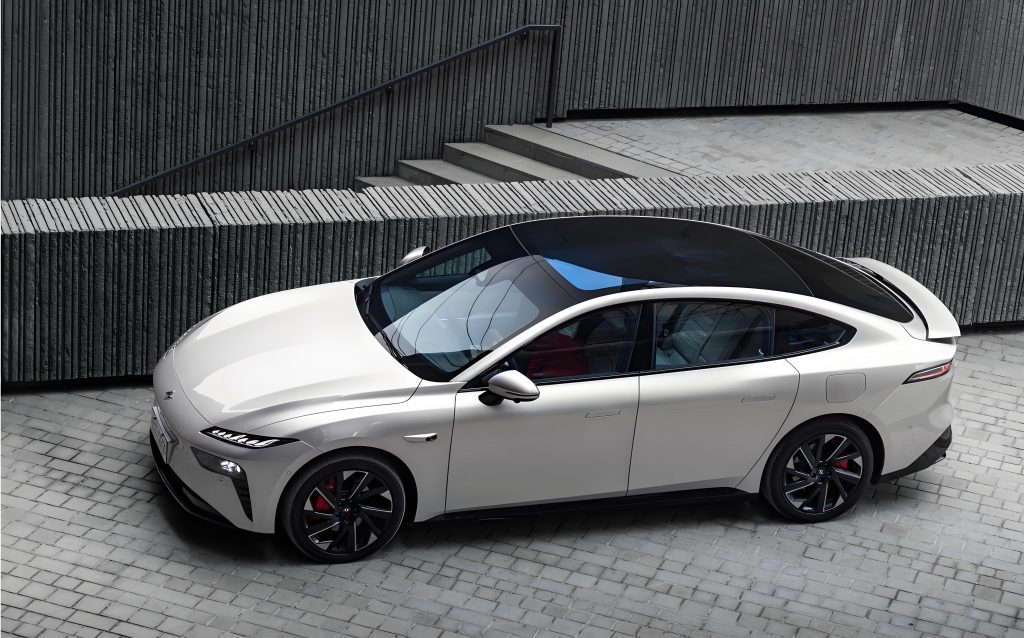
Charging strategies for rural electric vehicle car users are often opportunistic, occurring at home, farms, or public charging points during stops. If a charging facility is available at a destination, the electric vehicle car connects immediately and charges until reaching a target state-of-charge (SOC) or until the dwell time ends. The charging energy $E_c$ is given by:
$$E_c = P_c \cdot \eta \cdot \frac{SOC_{\text{target}} – SOC_{\text{arrive}}}{100} \cdot t_{\text{stay}}$$
where $P_c$ is charging power (slow charging at 7.5 kW for home/farming scenarios, fast charging at 60 kW for tourism scenarios), $\eta$ is efficiency, $SOC_{\text{arrive}}$ and $SOC_{\text{target}}$ are arrival and target SOC levels, and $t_{\text{stay}}$ is dwell time.
To assess the grid’s ability to accommodate electric vehicle car charging, I propose a spatio-temporal dynamic carrying capacity model based on the power regulation feasible domain of rural transformer districts. The feasible domain represents the range of power that can be safely exchanged between the grid and electric vehicle car charging loads while satisfying operational constraints. I define the baseline power of a transformer district as the total power demand from all resources except electric vehicle car, optimized for smooth operation considering controllable resources like energy storage, distributed photovoltaics (PV), wind turbines, shiftable loads, and curtailable loads.
The power regulation feasible domain assessment aims to maximize the total admissible electric vehicle car charging power across all time periods. The objective function is:
$$\max \sum_{t=1}^{T} (P_{\text{up},t} – P_{\text{down},t})$$
where $P_{\text{up},t}$ and $P_{\text{down},t}$ are the upper and lower bounds of the feasible domain at time $t$, $T$ is the scheduling horizon. These bounds are derived from the grid’s power exchange limits: $P_{\text{up},t} = P_{\text{max},t} – P_{\text{base},t}$ and $P_{\text{down},t} = P_{\text{min},t} – P_{\text{base},t}$, with $P_{\text{base},t}$ as the baseline load.
The constraints include AC power flow equations using the Distflow model. Let $P_{ij,t}$ and $Q_{ij,t}$ be the active and reactive power flows on branch $ij$ at time $t$, $U_{i,t}$ the voltage magnitude at node $i$, and $I_{ij,t}$ the current on branch $ij$. The power flow constraints are:
$$\sum_{k \in N(i)} (P_{ki,t} – R_{ki} I_{ki,t}^2) – \sum_{j \in M(i)} P_{ij,t} = P_{\text{inj},i,t}$$
$$\sum_{k \in N(i)} (Q_{ki,t} – X_{ki} I_{ki,t}^2) – \sum_{j \in M(i)} Q_{ij,t} = Q_{\text{inj},i,t}$$
$$U_{j,t}^2 = U_{i,t}^2 – 2(R_{ij} P_{ij,t} + X_{ij} Q_{ij,t}) + (R_{ij}^2 + X_{ij}^2) I_{ij,t}^2$$
$$I_{ij,t}^2 = \frac{P_{ij,t}^2 + Q_{ij,t}^2}{U_{i,t}^2}$$
for all branches $ij$ and time $t$. Node voltage constraints are $U_{\text{min},i} \leq U_{i,t} \leq U_{\text{max},i}$, branch current constraints are $I_{ij,t} \leq I_{\text{max},ij}$, and transformer loading constraints are $\sqrt{P_{\text{sub},t}^2 + Q_{\text{sub},t}^2} \leq \beta S_N$, where $S_N$ is the rated capacity and $\beta$ is a load factor. Other constraints include limits on PV and wind power outputs, controllable generation, shiftable loads, curtailable loads, and energy storage systems. For storage, the state-of-charge dynamics are:
$$SOC_{\text{ES},i,t+1} = SOC_{\text{ES},i,t} + (\eta_{\text{ch}} P_{\text{ch},i,t} – \frac{1}{\eta_{\text{dis}}} P_{\text{dis},i,t}) \Delta t$$
with bounds $SOC_{\text{min},i} \leq SOC_{\text{ES},i,t} \leq SOC_{\text{max},i}$.
To solve this model, I apply second-order cone (SOC) relaxation to handle non-convexities. By introducing variables $u_{i,t} = U_{i,t}^2$, $l_{ij,t} = I_{ij,t}^2$, $p_{ij,t} = P_{ij,t}$, and $q_{ij,t} = Q_{ij,t}$, the power flow equations become linear, and the constraint $l_{ij,t} u_{i,t} \geq p_{ij,t}^2 + q_{ij,t}^2$ is relaxed to a second-order cone constraint:
$$\left\| \begin{bmatrix} 2p_{ij,t} \\ 2q_{ij,t} \\ l_{ij,t} – u_{i,t} \end{bmatrix} \right\|_2 \leq l_{ij,t} + u_{i,t}$$
This transforms the problem into a mixed-integer second-order cone program (MISOCP), solvable with commercial solvers like CPLEX.
The electric vehicle car spatio-temporal dynamic carrying capacity is then defined as the set of all electric vehicle car charging scenarios that lie within the power regulation feasible domain. Formally, let $S_{F,EV}$ be the set of admissible electric vehicle car charging scenarios, $s_k \in \Omega_{EV}$ a specific scenario from the set of all possible scenarios, and $P_{EV}(s_k)$ the spatio-temporal charging power for scenario $s_k$. The carrying capacity condition is:
$$P_{\text{down}} \leq P_{\text{base}} + P_{EV}(s_k) \leq P_{\text{up}}$$
for all time periods and grid nodes. To compute this, I first generate electric vehicle car charging load scenarios based on the travel chain model, then evaluate them against the feasible domain bounds obtained from the optimization. The carrying capacity is visualized as a three-dimensional region showing maximum electric vehicle car numbers per node over time.
For case analysis, I use a modified IEEE 33-node system representing a rural grid, with distributed PV (50 kW per node) and electric vehicle car charging stations at nodes 13 and 30. I analyze three rural scenarios: summer farming, rural market day, and rural tourism. Table 4 summarizes the charging characteristics for these scenarios.
| Scenario | Charging Power | Peak Times | Typical Electric Vehicle Car Count at Peak |
|---|---|---|---|
| Summer Farming | 7.5 kW (slow) | 05:00-07:00, 12:00-14:00 | 27 (morning), 55 (noon) |
| Rural Market Day | 7.5 kW (slow) | 08:00 | ~67 (500 kW peak) |
| Rural Tourism | 60 kW (fast) | 12:00-14:00, 20:00-24:00 | ~5 (300 kW), ~6.7 (400 kW) |
In the summer farming scenario, I compare two carrying capacity assessment methods: Method 1 (static) and Method 2 (my spatio-temporal dynamic approach). Using actual data for PV output and residential load during summer farming, the PV output curve shows peaks around midday, and the load curve has evening peaks. The dynamic carrying capacity results are represented as a 3D surface where axes are time, electric vehicle car count at node 13, and electric vehicle car count at node 30. The surface defines the upper limit of admissible electric vehicle car numbers, with projections onto 2D planes revealing coupling between nodes and temporal variations. For example, when node 13 has 200 electric vehicle cars connected, node 30 can accommodate between 200 and 1400 electric vehicle cars, depending on other loads and PV generation. Static methods often overestimate or underestimate capacity, leading to risks of voltage violations or transformer overloads.
The dynamic carrying capacity varies hourly due to fluctuations in PV output, residential load, and electric vehicle car charging patterns. For instance, at 19:00, when PV output is low and residential load is high, the carrying capacity for node 30 drops to just 101 electric vehicle cars, whereas at other times, it can exceed 1000. This highlights the importance of temporal dynamics. Table 5 provides a sample of carrying capacity limits at different times for node 30 under the farming scenario.
| Time | Minimum Electric Vehicle Car Count (Lower Bound) | Maximum Electric Vehicle Car Count (Upper Bound) |
|---|---|---|
| 05:00 | 0 | 201 |
| 11:00 | 500 | 1150 |
| 14:00 | 0 | 121 |
| 19:00 | 0 | 101 |
| 23:00 | 0 | 800 |
The key advantage of my method is its ability to capture spatio-temporal couplings. For instance, increasing electric vehicle car connections at node 13 reduces the capacity at node 30, a relationship missed by static assessments. The feasible domain approach also integrates grid constraints comprehensively, ensuring safe operation under varying electric vehicle car penetration levels. To further illustrate, I derive the power flow equations in matrix form for the rural grid. Let $\mathbf{P}_t$ and $\mathbf{Q}_t$ be vectors of nodal injections, $\mathbf{U}_t$ the voltage magnitude squares, and $\mathbf{L}_t$ the branch current squares. The relaxed SOC model can be written as:
$$\mathbf{A} \mathbf{P}_t + \mathbf{B} \mathbf{Q}_t + \mathbf{C} \mathbf{L}_t \leq \mathbf{d}$$
$$\left\| \begin{bmatrix} 2\mathbf{P}_{ij,t} \\ 2\mathbf{Q}_{ij,t} \\ \mathbf{L}_{ij,t} – \mathbf{U}_{i,t} \end{bmatrix} \right\|_2 \leq \mathbf{L}_{ij,t} + \mathbf{U}_{i,t} \quad \forall ij$$
where $\mathbf{A}, \mathbf{B}, \mathbf{C}$ are coefficient matrices from grid topology and parameters, and $\mathbf{d}$ is a vector of limits.
In conclusion, my research provides a framework for modeling rural electric vehicle car charging behavior and assessing grid carrying capacity dynamically. By incorporating rural-specific travel patterns, environmental factors, and grid operational constraints into a feasible domain model, I enable more accurate and refined evaluations. This approach helps grid operators plan for electric vehicle car integration, mitigate risks of overloading, and optimize charging infrastructure deployment. Future work could focus on real-time control strategies to guide electric vehicle car charging based on spatio-temporal capacity, enhancing the utilization of rural grid resources while supporting the growth of electric vehicle car adoption in rural areas.
Throughout this article, I have emphasized the term “electric vehicle car” to align with the keyword requirement, though in practice, “electric vehicle” is commonly used. The methods and results demonstrate that rural grids can support significant electric vehicle car penetration if managed dynamically, paving the way for sustainable rural mobility. The integration of travel chain models, feasible domain theory, and optimization techniques offers a robust toolkit for addressing the challenges of electric vehicle car charging in rural settings, ultimately contributing to rural revitalization and energy transition goals.