
I present a complete study of position sensorless control for the permanent magnet synchronous motor in electric vehicle traction systems. My motivation is straightforward: the permanent magnet synchronous motor offers high efficiency, high power density, fast torque response, and a compact structure, but its high-performance field-oriented control depends strongly on accurate rotor position and speed information. Mechanical position sensors increase cost, wiring complexity, volume, and maintenance burden, and they can become unreliable under vibration, thermal cycling, and electromagnetic interference. Therefore, I investigate estimation and control strategies that remove the mechanical position sensor while preserving dynamic performance, steady-state accuracy, and robustness across the full speed range.
The permanent magnet synchronous motor is widely used in electric vehicle drive systems because it can produce high torque from a small volume and can operate with high efficiency over a broad operating region. However, the control problem is not merely a matter of replacing a sensor with an algorithm. At zero and low speed, the back electromotive force is very small, and the signal-to-noise ratio of position-related fundamental information becomes poor. At medium and high speed, the back electromotive force becomes strong, but parameter drift, sampling noise, inverter nonlinearity, and switching ripple can still corrupt the estimated position. A practical solution must therefore combine different estimation mechanisms and transition between them smoothly. I structure my work around this requirement.
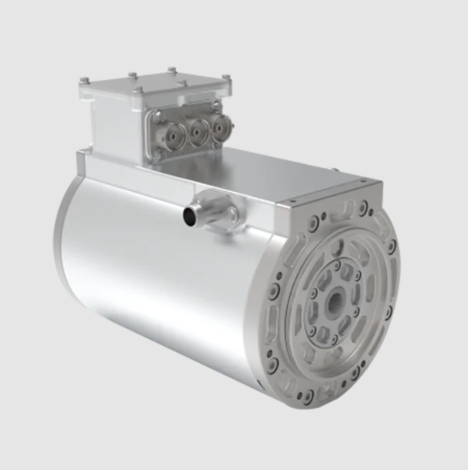
1. Research Background and Technical Challenge
I begin with the mathematical and physical reasons why sensorless control of the permanent magnet synchronous motor is difficult. The electromagnetic torque of the permanent magnet synchronous motor is produced by the interaction between the stator current and the permanent magnet field. In the rotor reference frame, the torque depends on the quadrature-axis current and, for interior permanent magnet machines, on the saliency-induced reluctance torque. Accurate coordinate transformation requires the rotor electrical angle. If the rotor angle is wrong, the current vector is misaligned, the torque per ampere decreases, and torque ripple increases. If the speed estimate is wrong, the speed loop and the decoupling terms become inconsistent. Thus, the estimation problem is central to the entire drive.
I classify the speed range into three regions. In the zero and low speed region, the permanent magnet synchronous motor has insufficient back electromotive force for model-based observers. In the medium and high speed region, back electromotive force is usable, but the observer must reject noise and parameter uncertainty. In the transition region, two estimation methods must be blended or switched without causing angle discontinuity or current shock. My design therefore uses high-frequency voltage injection at zero and low speed, a super-twisting sliding mode observer at medium and high speed, and a weighted transition strategy between them.
2. Mathematical Model of the Permanent Magnet Synchronous Motor
I first establish the permanent magnet synchronous motor model in several coordinate frames. The three-phase stationary model is useful for physical interpretation, the two-phase stationary model is convenient for observers, and the rotor synchronous model is convenient for vector control and model predictive current control.
The three-phase stator voltage equation is
$$
\begin{bmatrix}
u_a\\
u_b\\
u_c
\end{bmatrix}
=
R_s
\begin{bmatrix}
i_a\\
i_b\\
i_c
\end{bmatrix}
+
\frac{d}{dt}
\begin{bmatrix}
\psi_a\\
\psi_b\\
\psi_c
\end{bmatrix}
$$
For a permanent magnet synchronous motor with a sinusoidal permanent magnet flux distribution, the permanent magnet flux linkage in each phase can be written as
$$
\begin{aligned}
\psi_{fa}&=\psi_f\cos\theta_e\\
\psi_{fb}&=\psi_f\cos\left(\theta_e-\frac{2\pi}{3}\right)\\
\psi_{fc}&=\psi_f\cos\left(\theta_e+\frac{2\pi}{3}\right)
\end{aligned}
$$
After applying the Clarke transformation and neglecting the zero-sequence component for a balanced three-phase system, I obtain the two-phase stationary model:
$$
\begin{aligned}
u_\alpha&=R_s i_\alpha+\frac{d\psi_\alpha}{dt}\\
u_\beta&=R_s i_\beta+\frac{d\psi_\beta}{dt}
\end{aligned}
$$
For a surface-mounted permanent magnet synchronous motor, the inductance can be approximated as \(L_d \approx L_q \approx L_s\). The flux linkages in the stationary frame are then
$$
\begin{aligned}
\psi_\alpha&=L_s i_\alpha+\psi_f\cos\theta_e\\
\psi_\beta&=L_s i_\beta+\psi_f\sin\theta_e
\end{aligned}
$$
The back electromotive force components in the stationary frame are
$$
\begin{aligned}
e_\alpha&=-\omega_e\psi_f\sin\theta_e\\
e_\beta&=\omega_e\psi_f\cos\theta_e
\end{aligned}
$$
Therefore, the stationary-frame current dynamics can be written as
$$
\begin{aligned}
\frac{di_\alpha}{dt}&=-\frac{R_s}{L_s}i_\alpha+\frac{1}{L_s}u_\alpha-\frac{1}{L_s}e_\alpha\\
\frac{di_\beta}{dt}&=-\frac{R_s}{L_s}i_\beta+\frac{1}{L_s}u_\beta-\frac{1}{L_s}e_\beta
\end{aligned}
$$
In the rotor synchronous reference frame, the voltage equations are
$$
\begin{aligned}
u_d&=R_s i_d+L_d\frac{di_d}{dt}-\omega_e L_q i_q\\
u_q&=R_s i_q+L_q\frac{di_q}{dt}+\omega_e\left(L_d i_d+\psi_f\right)
\end{aligned}
$$
The electromagnetic torque of the permanent magnet synchronous motor is
$$
T_e=\frac{3}{2}p\left[\psi_f i_q+\left(L_d-L_q\right)i_d i_q\right]
$$
For a surface-mounted permanent magnet synchronous motor, \(L_d \approx L_q\), and the torque expression reduces to
$$
T_e=\frac{3}{2}p\psi_f i_q
$$
The mechanical dynamics are
$$
J\frac{d\omega_m}{dt}=T_e-T_L-B\omega_m
$$
with
$$
\omega_e=p\omega_m,\qquad \frac{d\theta_e}{dt}=\omega_e
$$
I summarize the principal symbols in the following table.
| Symbol | Meaning |
|---|---|
| \(u_d,u_q\) | Stator voltage components in the rotor reference frame |
| \(i_d,i_q\) | Stator current components in the rotor reference frame |
| \(L_d,L_q\) | Direct-axis and quadrature-axis inductances |
| \(R_s\) | Stator resistance |
| \(\psi_f\) | Permanent magnet flux linkage |
| \(\omega_e,\omega_m\) | Electrical and mechanical angular speeds |
| \(\theta_e\) | Rotor electrical angle |
| \(p\) | Number of pole pairs |
| \(J,B\) | Inertia and viscous damping |
| \(T_e,T_L\) | Electromagnetic torque and load torque |
3. Vector Control and Space Vector Pulse Width Modulation
I adopt field-oriented control with \(i_d=0\) as the baseline control structure for the permanent magnet synchronous motor. In this strategy, the direct-axis current is commanded to zero for a surface-mounted permanent magnet synchronous motor, and the quadrature-axis current is used to regulate torque. This choice simplifies the current control problem and is compatible with both proportional-integral current loops and model predictive current control. The speed loop generates the quadrature-axis current reference, while the direct-axis current reference is set to zero in the constant-torque region.
Space vector pulse width modulation is used to synthesize the reference voltage vector. The inverter has eight switching states, including six active vectors and two zero vectors. The sector of the reference voltage vector is determined from the signs of the stationary-frame voltage components. The dwell times of the active vectors are computed from the direct-current bus voltage and the sampling period. I summarize the sector logic in the following table.
| Sector index | Condition | Active vectors |
|---|---|---|
| I | \(u_\beta>0,\ \frac{\sqrt{3}}{2}u_\alpha-\frac{1}{2}u_\beta>0,\ -\frac{\sqrt{3}}{2}u_\alpha-\frac{1}{2}u_\beta\le 0\) | \(V_4,V_6\) |
| II | \(u_\beta>0,\ \frac{\sqrt{3}}{2}u_\alpha-\frac{1}{2}u_\beta\le 0,\ -\frac{\sqrt{3}}{2}u_\alpha-\frac{1}{2}u_\beta>0\) | \(V_2,V_6\) |
| III | \(u_\beta\le 0,\ \frac{\sqrt{3}}{2}u_\alpha-\frac{1}{2}u_\beta\le 0,\ -\frac{\sqrt{3}}{2}u_\alpha-\frac{1}{2}u_\beta>0\) | \(V_2,V_3\) |
| IV | \(u_\beta\le 0,\ \frac{\sqrt{3}}{2}u_\alpha-\frac{1}{2}u_\beta\le 0,\ -\frac{\sqrt{3}}{2}u_\alpha-\frac{1}{2}u_\beta\le 0\) | \(V_1,V_3\) |
| V | \(u_\beta\le 0,\ \frac{\sqrt{3}}{2}u_\alpha-\frac{1}{2}u_\beta>0,\ -\frac{\sqrt{3}}{2}u_\alpha-\frac{1}{2}u_\beta\le 0\) | \(V_1,V_5\) |
| VI | \(u_\beta>0,\ \frac{\sqrt{3}}{2}u_\alpha-\frac{1}{2}u_\beta>0,\ -\frac{\sqrt{3}}{2}u_\alpha-\frac{1}{2}u_\beta>0\) | \(V_5,V_6\) |
The active vector dwell times can be expressed in the general form
$$
T_x=\frac{\sqrt{3}T_s}{U_{dc}}u_\beta,\qquad
T_y=\frac{\sqrt{3}T_s}{U_{dc}}\left(\frac{\sqrt{3}}{2}u_\alpha+\frac{1}{2}u_\beta\right)
$$
where \(T_s\) is the sampling period and \(U_{dc}\) is the direct-current bus voltage. When the sum of the active times exceeds the sampling period, I apply an overmodulation limit:
$$
T_x’=\frac{T_x}{T_x+T_y}T_s,\qquad
T_y’=\frac{T_y}{T_x+T_y}T_s
$$
The zero-vector time is
$$
T_0=T_s-T_x’-T_y’
$$
These calculations are executed in real time by the digital signal processor. The resulting switching pattern drives the three-phase inverter and applies the required voltage vector to the permanent magnet synchronous motor.
4. Sensorless Control Framework Across the Full Speed Range
I design the sensorless control system as a speed-dependent framework. The permanent magnet synchronous motor behaves differently in different speed regions, and no single estimation method is optimal everywhere. The following table summarizes my design logic.
| Speed region | Dominant physical condition | Estimation method | Main challenge |
|---|---|---|---|
| Zero and low speed | Back electromotive force is very small; fundamental model observability is poor | Pulsating high-frequency voltage injection | Demodulation noise, additional loss, polarity identification |
| Medium and high speed | Back electromotive force is sufficient; model-based observation becomes feasible | Super-twisting sliding mode observer | Chattering suppression, parameter drift, noise rejection |
| Transition region | Both methods can operate but neither should dominate abruptly | Weighted fusion of angle and speed estimates | Angle continuity, current shock suppression, smooth torque |
I use the pulsating high-frequency voltage injection method at zero and low speed because it actively excites the saliency of the permanent magnet synchronous motor. The resulting high-frequency current contains rotor position information. I use the super-twisting sliding mode observer at medium and high speed because it reconstructs the back electromotive force from the stationary-frame current dynamics and provides strong robustness. I use weighted switching in the transition band because direct threshold switching can cause sudden angle jumps and torque transients.
5. Medium and High Speed Estimation with a Super-Twisting Sliding Mode Observer
I first consider the conventional sliding mode observer for the permanent magnet synchronous motor. The stationary-frame current observer is written as
$$
\begin{aligned}
\frac{d\hat{i}_\alpha}{dt}&=-\frac{R_s}{L_s}\hat{i}_\alpha+\frac{1}{L_s}u_\alpha-\frac{k}{L_s}\operatorname{sgn}\left(\hat{i}_\alpha-i_\alpha\right)\\
\frac{d\hat{i}_\beta}{dt}&=-\frac{R_s}{L_s}\hat{i}_\beta+\frac{1}{L_s}u_\beta-\frac{k}{L_s}\operatorname{sgn}\left(\hat{i}_\beta-i_\beta\right)
\end{aligned}
$$
When the current estimation error reaches the sliding surface, the equivalent back electromotive force can be reconstructed as
$$
\hat{e}_\alpha=k\operatorname{sgn}\left(\hat{i}_\alpha-i_\alpha\right),\qquad
\hat{e}_\beta=k\operatorname{sgn}\left(\hat{i}_\beta-i_\beta\right)
$$
The rotor position is then obtained from
$$
\hat{\theta}_e=-\arctan\left(\frac{\hat{e}_\alpha}{\hat{e}_\beta}\right)
$$
The conventional sliding mode observer is simple and robust, but the discontinuous sign function causes chattering. A low-pass filter is usually required, and the filter introduces phase lag that depends on speed. This phase lag must be compensated, and inaccurate compensation degrades current decoupling and torque quality. I therefore introduce the super-twisting sliding mode observer.
The super-twisting algorithm is a second-order sliding mode method. Its continuous and integral terms reduce chattering while preserving finite-time convergence and robustness. For the permanent magnet synchronous motor, I write the observer as
$$
\begin{aligned}
\frac{d\hat{i}_\alpha}{dt}
&=-\frac{R_s}{L_s}\hat{i}_\alpha+\frac{1}{L_s}u_\alpha
-\frac{k_1}{L_s}\left|\tilde{i}_\alpha\right|^{1/2}\operatorname{sgn}\left(\tilde{i}_\alpha\right)
-\frac{k_2}{L_s}\int\operatorname{sgn}\left(\tilde{i}_\alpha\right)dt\\
\frac{d\hat{i}_\beta}{dt}
&=-\frac{R_s}{L_s}\hat{i}_\beta+\frac{1}{L_s}u_\beta
-\frac{k_1}{L_s}\left|\tilde{i}_\beta\right|^{1/2}\operatorname{sgn}\left(\tilde{i}_\beta\right)
-\frac{k_2}{L_s}\int\operatorname{sgn}\left(\tilde{i}_\beta\right)dt
\end{aligned}
$$
where
$$
\tilde{i}_\alpha=\hat{i}_\alpha-i_\alpha,\qquad
\tilde{i}_\beta=\hat{i}_\beta-i_\beta
$$
After the sliding surface is reached, the equivalent back electromotive force estimates are
$$
\begin{aligned}
\hat{e}_\alpha
&=k_1\left|\tilde{i}_\alpha\right|^{1/2}\operatorname{sgn}\left(\tilde{i}_\alpha\right)
+k_2\int\operatorname{sgn}\left(\tilde{i}_\alpha\right)dt\\
\hat{e}_\beta
&=k_1\left|\tilde{i}_\beta\right|^{1/2}\operatorname{sgn}\left(\tilde{i}_\beta\right)
+k_2\int\operatorname{sgn}\left(\tilde{i}_\beta\right)dt
\end{aligned}
$$
I analyze stability using a Lyapunov function of the form
$$
V=\frac{1}{2}s^T s
$$
where \(s\) is the sliding variable. When the gains satisfy the super-twisting conditions, the derivative satisfies
$$
\dot{V}\le -\lambda V^{1/2}
$$
with \(\lambda>0\). This guarantees finite-time convergence to the sliding surface and bounded estimation error under bounded disturbance. The estimated rotor angle and speed are obtained from the reconstructed back electromotive force:
$$
\hat{\theta}_e=-\arctan\left(\frac{\hat{e}_\alpha}{\hat{e}_\beta}\right),\qquad
\hat{\omega}_e=\frac{\sqrt{\hat{e}_\alpha^2+\hat{e}_\beta^2}}{\psi_f}
$$
I compare the conventional sliding mode observer and the super-twisting sliding mode observer in the following table.
| Property | Conventional sliding mode observer | Super-twisting sliding mode observer |
|---|---|---|
| Sliding order | First order | Second order |
| Injection term | Discontinuous sign function | Continuous term plus integral term |
| Chattering | High | Low |
| Filter requirement | Usually required | Reduced or avoided |
| Phase compensation | Strongly speed dependent | Less sensitive |
| Robustness | Good | Strong |
| Position smoothness | Moderate | High |
6. Model Predictive Current Control for the Permanent Magnet Synchronous Motor
To improve current tracking and dynamic response, I combine the super-twisting sliding mode observer with model predictive current control. The permanent magnet synchronous motor current dynamics in the rotor reference frame are discretized using the forward Euler method:
$$
\begin{aligned}
i_d(k+1)
&=i_d(k)+\frac{T_s}{L_d}\left[u_d(k)-R_s i_d(k)+\omega_e L_q i_q(k)\right]\\
i_q(k+1)
&=i_q(k)+\frac{T_s}{L_q}\left[u_q(k)-R_s i_q(k)-\omega_e L_d i_d(k)-\omega_e\psi_f\right]
\end{aligned}
$$
For each of the eight inverter voltage vectors, I predict the next-step currents and evaluate a cost function. The cost function is
$$
J=\left(i_d^*-i_d^p(k+1)\right)^2+\left(i_q^*-i_q^p(k+1)\right)^2
$$
The voltage vector that minimizes \(J\) is selected and applied during the next sampling period. This replaces the conventional cascaded proportional-integral current loop with a rolling optimization process. The speed loop still generates \(i_q^*\), and \(i_d^*\) is set to zero. The advantages of model predictive current control for the permanent magnet synchronous motor include fast current tracking, explicit handling of voltage constraints, and reduced current ripple compared with a fixed-bandwidth proportional-integral current loop.
I compare proportional-integral current control and model predictive current control in the following table.
| Item | Proportional-integral current control | Model predictive current control |
|---|---|---|
| Control principle | Linear feedback with fixed gains | Model-based finite-set rolling optimization |
| Current tracking | Good but bandwidth limited | Fast and predictive |
| Constraint handling | Requires anti-windup and limits | Can be embedded in the cost function |
| Parameter sensitivity | Moderate | Depends on model accuracy but can be compensated |
| Current ripple | Higher under disturbance | Lower in the tested conditions |
| Complexity | Low | Moderate |
In my simulation comparison, the super-twisting sliding mode observer with model predictive current control achieves smaller speed overshoot, lower torque ripple, and smoother three-phase currents than the same observer with proportional-integral current control. The position estimation error is also reduced. I describe the main outcomes in a later section.
7. Zero and Low Speed Estimation with Pulsating High-Frequency Voltage Injection
At zero and low speed, the back electromotive force of the permanent magnet synchronous motor is approximately zero, so the fundamental model loses observability. I therefore inject a pulsating high-frequency voltage into the estimated direct axis. The injection signal is
$$
u_{\hat{d}h}=u_h\cos\left(\omega_h t\right),\qquad
u_{\hat{q}h}=0
$$
The high-frequency voltage excites the saliency of the permanent magnet synchronous motor. The inductance matrix in the stationary frame is
$$
L_{\alpha\beta}
=
\begin{bmatrix}
L+\Delta L\cos 2\theta_e & \Delta L\sin 2\theta_e\\
\Delta L\sin 2\theta_e & L-\Delta L\cos 2\theta_e
\end{bmatrix}
$$
where
$$
L=\frac{L_d+L_q}{2},\qquad
\Delta L=\frac{L_q-L_d}{2}
$$
When the estimated rotor frame differs from the actual rotor frame by
$$
\Delta\theta=\hat{\theta}_e-\theta_e
$$
the high-frequency current components in the estimated frame become
$$
\begin{aligned}
i_{\hat{d}h}
&=\frac{u_h}{\omega_h\left(L^2-\Delta L^2\right)}
\left(L+\Delta L\cos 2\Delta\theta\right)\sin\left(\omega_h t\right)\\
i_{\hat{q}h}
&=\frac{u_h}{\omega_h\left(L^2-\Delta L^2\right)}
\Delta L\sin 2\Delta\theta\sin\left(\omega_h t\right)
\end{aligned}
$$
The quadrature-axis high-frequency current contains the position error. I demodulate it by multiplying with \(\sin(\omega_h t)\) and applying a low-pass filter:
$$
\varepsilon
=i_{\hat{q}h}\sin\left(\omega_h t\right)
\xrightarrow{\text{LPF}}
M\sin 2\Delta\theta
\approx 2M\Delta\theta
$$
where
$$
M=\frac{u_h\Delta L}{2\omega_h\left(L^2-\Delta L^2\right)}
$$
For small errors, the demodulated signal is proportional to the position error. I then use a phase-locked loop to drive the error to zero:
$$
\Delta\hat{\omega}_e=K_p\varepsilon+K_i\int\varepsilon dt
$$
$$
\hat{\theta}_e=\int\hat{\omega}_e dt
$$
Because the saliency-based position estimate is ambiguous by 180 electrical degrees, I also identify the north and south poles. I inject two voltage pulses of equal amplitude and opposite polarity along the estimated direct axis. Magnetic saturation causes the direct-axis inductance to decrease when the pulse magnetizes the rotor in the north direction and to increase when the pulse magnetizes it in the south direction. I sample the high-frequency current at two instants:
$$
i_{dh1}=\hat{i}_{dh}\sin\left(\frac{\pi}{2}\right),\qquad
i_{dh2}=\hat{i}_{dh}\sin\left(\frac{3\pi}{2}\right)
$$
If \(i_{dh1}>i_{dh2}\), the estimated direct axis aligns with the north pole. If \(i_{dh1}<i_{dh2}\), \(\pi\)="" add="" aligns="" and="" angle.="" axis="" below.
| Condition | Pole identification | Angle correction | |
|---|---|---|---|
| \(i_{dh1}>i_{dh2}\) | North pole | \(\hat{\theta}_e=\hat{\theta}_e\) | |
| \(i_{dh1}<i_{dh2}\) | South pole | \(\hat{\theta}_e=\hat{\theta}_e+\pi\) |
I use the pulsating high-frequency voltage injection method only at zero and low speed. Continuous injection increases copper loss, iron loss, acoustic noise, and current harmonics. Therefore, I transition to the super-twisting sliding mode observer as speed rises. The injection parameters must be chosen so that the high-frequency response is measurable but the additional loss is acceptable. In my design, the injection frequency lies in the kilohertz range, and the injection amplitude is a small fraction of the rated voltage.
8. Full-Speed Transition Strategy
I use a weighted transition strategy for the permanent magnet synchronous motor. A hysteresis switch is simple, but it can cause abrupt angle changes and current shocks. A weighted blend maintains continuity. I define two speed thresholds, \(\omega_1\) and \(\omega_2\). Below \(\omega_1\), the high-frequency injection method provides the angle and speed. Above \(\omega_2\), the super-twisting sliding mode observer provides the angle and speed. Between \(\omega_1\) and \(\omega_2\), the two estimates are blended.
The blended angle and speed are
$$
\hat{\theta}_e=\mu_1\hat{\theta}_{e,HFSI}+\mu_2\hat{\theta}_{e,ST-SMO}
$$
$$
\hat{\omega}_e=\mu_1\hat{\omega}_{e,HFSI}+\mu_2\hat{\omega}_{e,ST-SMO}
$$
with
$$
\mu_1+\mu_2=1
$$
The weighting coefficient for the high-frequency injection method is
$$
\mu_1=
\begin{cases}
1, & |\hat{\omega}_e|\le \omega_1\\[4pt]
\dfrac{\omega_2-|\hat{\omega}_e|}{\omega_2-\omega_1}, & \omega_1<|\hat{\omega}_e|<\omega_2\\[8pt]
0, & |\hat{\omega}_e|\ge \omega_2
\end{cases}
$$
and
$$
\mu_2=1-\mu_1
$$
I summarize the transition logic in the following table.
| Speed condition | High-frequency injection weight | Super-twisting observer weight | Active estimation |
|---|---|---|---|
| \(|\hat{\omega}_e|\le \omega_1\) | \(\mu_1=1\) | \(\mu_2=0\) | High-frequency injection only |
| \(\omega_1<|\hat{\omega}_e|<\omega_2\) | \(\mu_1=\frac{\omega_2-|\hat{\omega}_e|}{\omega_2-\omega_1}\) | \(\mu_2=\frac{|\hat{\omega}_e|-\omega_1}{\omega_2-\omega_1}\) | Weighted fusion |
| \(|\hat{\omega}_e|\ge \omega_2\) | \(\mu_1=0\) | \(\mu_2=1\) | Super-twisting observer only |
In my design, I set \(\omega_1=300\ \text{r/min}\) and \(\omega_2=750\ \text{r/min}\). This band is wide enough to avoid repeated switching and narrow enough to reduce the duration of high-frequency injection. The weighted transition preserves angle continuity and reduces current shock during acceleration and deceleration. I also apply phase alignment before blending so that the two angle estimates refer to the same electrical cycle. Without phase alignment, a weighted sum of angles can produce an incorrect intermediate angle even if both estimates are close to the true angle.
9. Simulation Model and Control Structure
I build a full-speed sensorless control model for the permanent magnet synchronous motor. The model includes the permanent magnet synchronous motor, the three-phase inverter, space vector pulse width modulation, the speed loop, the current loop, the high-frequency injection branch, the super-twisting sliding mode observer, and the weighted transition module. The control structure follows the logic below.
| Block | Function |
|---|---|
| Speed controller | Generates the quadrature-axis current reference from the speed error |
| Current controller | Model predictive current control selects the optimal voltage vector |
| Coordinate transformation | Uses the estimated rotor angle for Park and inverse Park transformations |
| Space vector pulse width modulation | Generates switching signals for the inverter |
| High-frequency injection | Estimates rotor position at zero and low speed |
| Super-twisting sliding mode observer | Estimates rotor position and speed at medium and high speed |
| Weighted transition | Blends the two estimation outputs according to speed |
The permanent magnet synchronous motor parameters used in my study are listed below.
| Parameter | Value |
|---|---|
| Rated voltage | \(380\ \text{V}\) |
| Rated speed | \(1500\ \text{r/min}\) |
| Number of pole pairs | \(4\) |
| Stator inductance | \(0.0085\ \text{H}\) |
| Stator resistance | \(2.875\ \Omega\) |
| Permanent magnet flux linkage | \(0.5\ \text{Wb}\) |
| Inertia | \(0.025\ \text{kg}\cdot\text{m}^2\) |
10. Simulation Results and Discussion
I first compare the conventional sliding mode observer and the super-twisting sliding mode observer under a speed reference of \(1000\ \text{r/min}\). The permanent magnet synchronous motor starts with no load, and a load torque of \(20\ \text{N}\cdot\text{m}\) is applied at \(0.1\ \text{s}\). The super-twisting observer reduces chattering and recovers faster after the load step. The estimated speed is smoother, and the position error is smaller. This confirms that the second-order sliding mode structure is better suited to the permanent magnet synchronous motor at medium and high speed.
I then compare two current control methods: super-twisting observer with proportional-integral current control and super-twisting observer with model predictive current control. The model predictive current control reduces the maximum speed deviation during startup. In my simulation, the maximum speed deviation is approximately \(13\ \text{r/min}\) with proportional-integral current control and approximately \(11\ \text{r/min}\) with model predictive current control. The torque ripple and three-phase current ripple are also lower with model predictive current control. The position error is approximately \(0.072\ \text{rad}\) with proportional-integral current control and approximately \(0.05\ \text{rad}\) with model predictive current control.
For zero and low speed, I test the high-frequency injection method with and without model predictive current control. The initial speed is \(100\ \text{r/min}\), and the speed rises to \(150\ \text{r/min}\) at \(0.1\ \text{s}\). The speed error is reduced from about \(0.21\ \text{r/min}\) to about \(0.13\ \text{r/min}\) when model predictive current control is used. This shows that the combination of high-frequency injection and model predictive current control improves low-speed estimation smoothness for the permanent magnet synchronous motor.
I then test the full-speed range. The permanent magnet synchronous motor starts at \(100\ \text{r/min}\), accelerates to \(1000\ \text{r/min}\), and then operates under load disturbance. The estimated speed tracks the actual speed with an error within approximately \(\pm 1\ \text{r/min}\) in steady state. The estimated rotor position follows the actual position with small error. The transition from high-frequency injection to the super-twisting observer is smooth, and no large current shock appears. I summarize the key simulation comparisons below.
| Case | Control method | Key observation |
|---|---|---|
| Medium and high speed | Conventional sliding mode observer | Noticeable chattering in estimated speed and position |
| Medium and high speed | Super-twisting sliding mode observer | Reduced chattering, faster recovery after load step |
| Medium and high speed | Super-twisting observer with proportional-integral current control | Speed overshoot \(13\ \text{r/min}\), position error \(0.072\ \text{rad}\) |
| Medium and high speed | Super-twisting observer with model predictive current control | Speed overshoot \(11\ \text{r/min}\), position error \(0.05\ \text{rad}\) |
| Zero and low speed | High-frequency injection without model predictive current control | Speed error \(0.21\ \text{r/min}\) |
| Zero and low speed | High-frequency injection with model predictive current control | Speed error \(0.13\ \text{r/min}\) |
11. Hardware and Software Implementation
I implement the sensorless control system for the permanent magnet synchronous motor on a modular hardware platform. The control unit and the power unit are separated to reduce electromagnetic interference and to simplify debugging. The power unit contains the intelligent power module, the gate drive and isolation circuits, and the direct-current bus. The control unit contains the digital signal processor, the auxiliary power supply, the voltage and current sampling circuits, and the position and speed detection interface.
The digital signal processor executes the control algorithm, samples the direct-current bus voltage, the direct-current bus current, and the three-phase currents, and generates the pulse width modulation signals. The isolation drive circuit uses high-speed optocouplers to transfer the pulse width modulation signals from the control side to the power side. The auxiliary power supply provides multiple voltage rails for the gate drivers, sensors, signal conditioning circuits, and digital logic. The voltage and current sampling circuits use Hall-effect sensors and conditioning amplifiers to scale the measured signals into the analog-to-digital converter range. The position and speed detection module uses an incremental optical encoder only as a reference for validating the estimated angle and speed; it does not participate in the closed-loop control.
I summarize the hardware modules and their functions below.
| Module | Main function |
|---|---|
| Digital signal processor control circuit | Executes estimation, speed control, current control, and pulse width modulation |
| Isolated gate drive circuit | Transfers pulse width modulation signals and isolates the power stage |
| Auxiliary power supply | Provides isolated and regulated voltage rails |
| Direct-current bus voltage sampling | Measures the direct-current bus voltage for control and protection |
| Direct-current bus current sampling | Measures the direct-current bus current for protection |
| Alternating-current voltage sampling | Measures the three-phase voltage for observation and protection |
| Alternating-current current sampling | Measures the three-phase current for current control |
| Encoder interface | Provides reference position and speed for validation only |
The software is developed in an integrated development environment. The main program initializes the clock, the input-output ports, the analog-to-digital converter, the pulse width modulation module, the quadrature encoder pulse module, and the communication interface. After initialization, the main loop manages the system state and the start-stop commands. The interrupt service routine performs the critical real-time tasks: current sampling, coordinate transformation, speed estimation, position estimation, current prediction, cost function evaluation, and pulse width modulation update. A separate protection routine shuts down the pulse width modulation outputs when overvoltage or overcurrent is detected.
The speed control algorithm subroutine follows this sequence:
| Step | Operation |
|---|---|
| 1 | Read the speed reference and the estimated speed |
| 2 | Compute the quadrature-axis current reference through the speed controller |
| 3 | Set the direct-axis current reference to zero |
| 4 | Predict the next-step currents for all inverter voltage vectors |
| 5 | Evaluate the cost function and select the optimal voltage vector |
| 6 | Apply the switching state through space vector pulse width modulation |
| 7 | Update the observer and the transition weights |
12. Experimental Validation
I build an experimental platform for the permanent magnet synchronous motor and conduct tests in the zero and low speed region, the medium and high speed region, and the full-speed region. The encoder is used only to compare the estimated values with the actual values. The control algorithms run on the digital signal processor in real time.
In the zero and low speed test, the permanent magnet synchronous motor starts with no load at \(100\ \text{r/min}\). The speed is increased to \(200\ \text{r/min}\) at \(0.1\ \text{s}\) and then reduced to \(150\ \text{r/min}\) at \(0.2\ \text{s}\). The estimated speed and rotor position track the actual values well during acceleration and deceleration. In the medium and high speed test, the motor starts at \(1000\ \text{r/min}\), a load torque of \(10\ \text{N}\cdot\text{m}\) is applied at \(0.1\ \text{s}\), and the speed reference is changed to \(1200\ \text{r/min}\) and then to \(800\ \text{r/min}\). The estimated speed follows the actual speed closely, and the system recovers quickly after the load step. The estimated rotor position tracks the actual rotor position. In the full-speed test, the motor starts at \(100\ \text{r/min}\) and accelerates to \(1000\ \text{r/min}\). The estimated speed and angle remain stable through the transition region.
I summarize the experimental conditions and observations below.
| Test | Speed command | Load condition | Observation |
|---|---|---|---|
| Zero and low speed | \(100\rightarrow 200\rightarrow 150\ \text{r/min}\) | No load | Estimated speed and position follow actual values |
| Medium and high speed | \(1000\rightarrow 1200\rightarrow 800\ \text{r/min}\) | \(10\ \text{N}\cdot\text{m}\) step at \(0.1\ \text{s}\) | Fast recovery, small estimation error |
| Full speed | \(100\rightarrow 1000\ \text{r/min}\) | No load | Smooth transition, stable full-speed operation |
The experimental results confirm that the permanent magnet synchronous motor can operate without a mechanical position sensor across the tested speed range. The high-frequency injection method provides reliable position information at zero and low speed. The super-twisting sliding mode observer provides smooth and robust estimation at medium and high speed. The weighted transition strategy prevents angle discontinuity and reduces current shock. The model predictive current control improves current tracking and reduces torque ripple.
13. Key Contributions and Engineering Value
My work contributes to the sensorless control of the permanent magnet synchronous motor in electric vehicle drives in several ways. First, I combine a super-twisting sliding mode observer with model predictive current control for the medium and high speed region. The second-order sliding mode structure reduces chattering, and the predictive current controller improves current tracking and dynamic response. Second, I use pulsating high-frequency voltage injection with north-south pole identification for the zero and low speed region. This provides reliable starting and low-speed operation despite the weak back electromotive force of the permanent magnet synchronous motor. Third, I design a weighted full-speed transition strategy that blends the two estimation methods and avoids abrupt switching. Fourth, I implement the complete control system on a modular hardware platform and validate it experimentally.
The engineering value is clear. Removing the mechanical position sensor reduces cost, wiring, volume, and maintenance. It also improves tolerance to vibration and electromagnetic interference. For the permanent magnet synchronous motor, sensorless control can increase the integration level of the electric drive system and improve reliability under harsh vehicle operating conditions. The combination of high-frequency injection, super-twisting sliding mode observation, model predictive current control, and weighted transition provides a practical path toward full-speed sensorless operation.
14. Limitations and Future Work
I also recognize several limitations. Parameter drift, magnetic saturation, inverter nonlinearity, and sampling delay can still degrade estimation accuracy. The high-frequency injection method introduces additional loss, acoustic noise, and current harmonics. The transition strategy must be tuned carefully to avoid phase misalignment between the two angle estimates. The experimental validation covers several key operating conditions, but long-term durability and real-road load profiles require further study.
In future work, I plan to improve the adaptive capability of the observer and the injection method under parameter variation. I will investigate lower-loss injection waveforms and more efficient demodulation schemes. I will also develop a confidence-based fusion mechanism for the full-speed transition, so that the weighting coefficients depend not only on speed but also on estimation quality. Finally, I will integrate the sensorless permanent magnet synchronous motor drive with vehicle-level energy management and thermal management and conduct longer-term tests under realistic driving cycles.
15. Concluding Summary
I have presented a full-speed sensorless control system for the permanent magnet synchronous motor. The system uses pulsating high-frequency voltage injection at zero and low speed, a super-twisting sliding mode observer at medium and high speed, and a weighted transition strategy between the two regions. The permanent magnet synchronous motor model is established in the three-phase stationary frame, the two-phase stationary frame, and the rotor synchronous frame. Vector control with \(i_d=0\) and space vector pulse width modulation form the baseline drive structure. Model predictive current control replaces the conventional proportional-integral current loop and improves current tracking and dynamic response. The super-twisting sliding mode observer reduces chattering and improves position and speed estimation. The high-frequency injection method provides reliable position information when the back electromotive force of the permanent magnet synchronous motor is too small for fundamental-model observers.
Simulation and experimental results show that the proposed method achieves smooth speed tracking, accurate rotor position estimation, and stable operation under acceleration, deceleration, and load disturbance. The full-speed transition strategy provides continuity between the zero and low speed region and the medium and high speed region. The permanent magnet synchronous motor drive can therefore operate without a mechanical position sensor while maintaining good dynamic and steady-state performance. I conclude that the proposed structure is a practical and effective solution for electric vehicle traction systems that require high efficiency, high power density, and high reliability.