
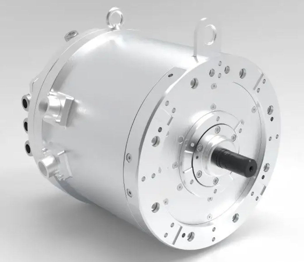
In my research, I focus on the sensorless control of a PMSM electric motor for electric vehicle traction applications. The transition toward electrified transportation has placed strong demands on drive systems with high efficiency, high power density, and high reliability. A PMSM electric motor is widely regarded as a preferred solution because it offers high torque density, fast dynamic response, and high efficiency. However, its vector control depends heavily on accurate rotor position and speed information. Mechanical position sensors increase cost, wiring complexity, and integration difficulty, and they may suffer from reliability degradation under vibration, thermal cycling, and electromagnetic interference. Therefore, I investigate a full-speed-range sensorless control strategy for a PMSM electric motor, covering zero and low speed operation, medium and high speed operation, and smooth switching between these regions.
The main objective of my work is to reduce dependence on mechanical position sensors while preserving dynamic performance and robustness. I establish a mathematical model of the PMSM electric motor in different coordinate systems, design a super-twisting sliding mode observer for medium and high speed estimation, apply pulsating high-frequency voltage injection for zero and low speed estimation, combine these methods with model predictive current control, and implement a weighted switching strategy for full-speed-range operation. I validate the proposed methods through simulations and experiments. The results indicate that the proposed sensorless control scheme can achieve accurate rotor position and speed estimation, smooth acceleration and deceleration, and strong disturbance rejection for a PMSM electric motor in electric vehicle applications.
Mathematical Model of the PMSM Electric Motor
To design a sensorless control system, I first establish the mathematical model of the PMSM electric motor. The model is expressed in the three-phase stationary coordinate system, the two-phase stationary coordinate system, and the synchronous rotating coordinate system. These representations provide the foundation for field-oriented control and observer design.
Three-Phase Stationary Coordinate System
In the three-phase stationary coordinate system, the stator voltage equation of the PMSM electric motor can be written as
$$ \begin{bmatrix} u_a \\ u_b \\ u_c \end{bmatrix} = R_s \begin{bmatrix} i_a \\ i_b \\ i_c \end{bmatrix} + \frac{d}{dt} \begin{bmatrix} \psi_a \\ \psi_b \\ \psi_c \end{bmatrix} $$
where \(u_a, u_b, u_c\) are the three-phase stator voltages, \(i_a, i_b, i_c\) are the three-phase stator currents, \(R_s\) is the stator resistance, and \(\psi_a, \psi_b, \psi_c\) are the three-phase stator flux linkages. The flux linkage equation is
$$ \begin{bmatrix} \psi_a \\ \psi_b \\ \psi_c \end{bmatrix} = \mathbf{L}(\theta_e) \begin{bmatrix} i_a \\ i_b \\ i_c \end{bmatrix} + \begin{bmatrix} \psi_{fa}(\theta_e) \\ \psi_{fb}(\theta_e) \\ \psi_{fc}(\theta_e) \end{bmatrix} $$
where \(\theta_e\) is the electrical rotor angle. For an ideal PMSM electric motor with sinusoidal back electromotive force, the permanent magnet flux linkage components can be expressed as
$$ \psi_{fa} = \psi_f \cos \theta_e, \quad \psi_{fb} = \psi_f \cos\left(\theta_e – \frac{2\pi}{3}\right), \quad \psi_{fc} = \psi_f \cos\left(\theta_e + \frac{2\pi}{3}\right) $$
where \(\psi_f\) is the permanent magnet flux linkage amplitude.
Two-Phase Stationary Coordinate System
By applying the Clarke transformation, I obtain the model in the \(\alpha-\beta\) stationary coordinate system. Under the assumption of a symmetric three-phase system without neutral connection, the zero-sequence component is ignored. The voltage equation becomes
$$ u_\alpha = R_s i_\alpha + \frac{d\psi_\alpha}{dt}, \quad u_\beta = R_s i_\beta + \frac{d\psi_\beta}{dt} $$
For a surface-mounted PMSM electric motor, the d-axis and q-axis inductances are approximately equal, and the flux linkages can be written as
$$ \psi_\alpha = L i_\alpha + \psi_f \cos\theta_e, \quad \psi_\beta = L i_\beta + \psi_f \sin\theta_e $$
Substituting these expressions into the voltage equation yields the current state equation:
$$ \frac{di_\alpha}{dt} = -\frac{R_s}{L} i_\alpha + \frac{1}{L} u_\alpha – \frac{1}{L} e_\alpha, \quad \frac{di_\beta}{dt} = -\frac{R_s}{L} i_\beta + \frac{1}{L} u_\beta – \frac{1}{L} e_\beta $$
where the back electromotive force components are
$$ e_\alpha = -\omega_e \psi_f \sin\theta_e, \quad e_\beta = \omega_e \psi_f \cos\theta_e $$
and \(\omega_e\) is the electrical angular speed. The mechanical motion equation is
$$ J \frac{d\omega_m}{dt} = T_e – T_L – B\omega_m, \quad \omega_e = p \omega_m $$
where \(J\) is the moment of inertia, \(B\) is the viscous damping coefficient, \(\omega_m\) is the mechanical angular speed, \(T_L\) is the load torque, and \(p\) is the number of pole pairs.
Synchronous Rotating Coordinate System
In the d-q synchronous rotating coordinate system, the voltage equations of the PMSM electric motor are
$$ u_d = R_s i_d + \frac{d\psi_d}{dt} – \omega_e \psi_q, \quad u_q = R_s i_q + \frac{d\psi_q}{dt} + \omega_e \psi_d $$
The flux linkage equations are
$$ \psi_d = L_d i_d + \psi_f, \quad \psi_q = L_q i_q $$
Substituting the flux linkages into the voltage equations gives
$$ u_d = R_s i_d + L_d \frac{di_d}{dt} – \omega_e L_q i_q, \quad u_q = R_s i_q + L_q \frac{di_q}{dt} + \omega_e (L_d i_d + \psi_f) $$
The electromagnetic torque is
$$ T_e = \frac{3}{2} p \left[ \psi_f i_q + (L_d – L_q) i_d i_q \right] $$
For a surface-mounted PMSM electric motor with \(L_d \approx L_q\), the torque expression simplifies to
$$ T_e = \frac{3}{2} p \psi_f i_q $$
The relationship between electrical and mechanical angular speed is
$$ \omega_e = p \omega_m, \quad \frac{d\theta_e}{dt} = \omega_e $$
Table 1 summarizes the variables and parameters used in the PMSM electric motor model.
| Symbol | Description | Unit |
|---|---|---|
| \(u_d, u_q\) | d-axis and q-axis stator voltages | V |
| \(i_d, i_q\) | d-axis and q-axis stator currents | A |
| \(L_d, L_q\) | d-axis and q-axis inductances | H |
| \(R_s\) | Stator resistance | \(\Omega\) |
| \(\psi_f\) | Permanent magnet flux linkage | Wb |
| \(\omega_e, \omega_m\) | Electrical and mechanical angular speed | rad/s |
| \(\theta_e\) | Electrical rotor angle | rad |
| \(T_e, T_L\) | Electromagnetic torque and load torque | N·m |
| \(J\) | Moment of inertia | kg·m² |
| \(p\) | Number of pole pairs | — |
Vector Control and Space Vector Pulse Width Modulation
For the PMSM electric motor, I adopt field-oriented control with \(i_d = 0\). This strategy is simple and effective for surface-mounted machines. The q-axis current directly controls the electromagnetic torque, while the d-axis current is regulated to zero to minimize copper loss. The overall vector control system includes speed control, current control, coordinate transformation, and space vector pulse width modulation (SVPWM).
SVPWM Implementation
The SVPWM technique determines the sector of the reference voltage vector and calculates the action times of the basic voltage vectors. The reference voltage vector components in the \(\alpha-\beta\) plane are \(u_\alpha\) and \(u_\beta\). I define three auxiliary variables \(A\), \(B\), and \(C\) as
$$ A = 1 \text{ if } u_\beta > 0, \text{ else } A = 0 $$
$$ B = 1 \text{ if } \frac{\sqrt{3}}{2} u_\alpha – \frac{1}{2} u_\beta > 0, \text{ else } B = 0 $$
$$ C = 1 \text{ if } -\frac{\sqrt{3}}{2} u_\alpha – \frac{1}{2} u_\beta > 0, \text{ else } C = 0 $$
The sector number is determined by \(N = 4C + 2B + A\). Table 2 lists the correspondence between \(N\) and the sector.
| \(N\) | 3 | 1 | 5 | 4 | 6 | 2 |
|---|---|---|---|---|---|---|
| Sector | I | II | III | IV | V | VI |
The action times of the non-zero vectors \(T_4\) and \(T_6\), and the zero vector \(T_0\), are calculated as follows. Let
$$ X = \frac{\sqrt{3} T_s}{U_{dc}} u_\beta, \quad Y = \frac{T_s}{U_{dc}} \left( \frac{3}{2} u_\alpha + \frac{\sqrt{3}}{2} u_\beta \right), \quad Z = \frac{T_s}{U_{dc}} \left( -\frac{3}{2} u_\alpha + \frac{\sqrt{3}}{2} u_\beta \right) $$
where \(T_s\) is the switching period and \(U_{dc}\) is the DC bus voltage. The action times for each sector are given in Table 3.
| \(N\) | 1 | 2 | 3 | 4 | 5 | 6 |
|---|---|---|---|---|---|---|
| \(T_4\) | \(Z\) | \(Y\) | \(-Z\) | \(-X\) | \(X\) | \(-Y\) |
| \(T_6\) | \(Y\) | \(-X\) | \(X\) | \(Z\) | \(-Y\) | \(-Z\) |
| \(T_0\) | \(T_0 = \frac{T_s – T_4 – T_6}{2}\) | |||||
If \(T_4 + T_6 > T_s\), the action times are adjusted as
$$ T_4′ = \frac{T_4}{T_4 + T_6} T_s, \quad T_6′ = \frac{T_6}{T_4 + T_6} T_s $$
The switching time instants are then obtained by
$$ T_a = \frac{T_s – T_4′ – T_6′}{4}, \quad T_b = T_a + \frac{T_4′}{2}, \quad T_c = T_b + \frac{T_6′}{2} $$
The final PWM signals are generated by comparing these time instants with a triangular carrier. This SVPWM implementation provides high DC voltage utilization and low harmonic distortion for the PMSM electric motor drive.
Medium and High Speed Rotor Position Estimation
At medium and high speeds, the back electromotive force of the PMSM electric motor is sufficiently large, so model-based observers can be used for rotor position and speed estimation. I design a super-twisting sliding mode observer to reduce chattering and improve estimation accuracy.
Traditional Sliding Mode Observer
In the \(\alpha-\beta\) stationary coordinate system, the current state equations of the PMSM electric motor are
$$ \frac{di_\alpha}{dt} = -\frac{R_s}{L_s} i_\alpha + \frac{1}{L_s} u_\alpha – \frac{1}{L_s} e_\alpha, \quad \frac{di_\beta}{dt} = -\frac{R_s}{L_s} i_\beta + \frac{1}{L_s} u_\beta – \frac{1}{L_s} e_\beta $$
A conventional sliding mode observer is constructed as
$$ \frac{d\hat{i}_\alpha}{dt} = -\frac{R_s}{L_s} \hat{i}_\alpha + \frac{1}{L_s} u_\alpha – \frac{k}{L_s} \operatorname{sgn}(\hat{i}_\alpha – i_\alpha) $$
$$ \frac{d\hat{i}_\beta}{dt} = -\frac{R_s}{L_s} \hat{i}_\beta + \frac{1}{L_s} u_\beta – \frac{k}{L_s} \operatorname{sgn}(\hat{i}_\beta – i_\beta) $$
where \(k\) is the sliding mode gain. When the system reaches the sliding surface, the equivalent control yields the back electromotive force estimates:
$$ \hat{e}_\alpha = k \operatorname{sgn}(\hat{i}_\alpha – i_\alpha), \quad \hat{e}_\beta = k \operatorname{sgn}(\hat{i}_\beta – i_\beta) $$
The rotor position is then calculated by
$$ \hat{\theta}_e = -\arctan\left( \frac{\hat{e}_\alpha}{\hat{e}_\beta} \right) $$
Because the sign function introduces high-frequency chattering, a low-pass filter is usually needed. However, the filter introduces phase delay, which requires compensation. The compensated position is
$$ \hat{\theta}_{e,c} = \hat{\theta}_e + \arctan\left( \frac{\hat{\omega}_e}{\omega_c} \right) $$
where \(\omega_c\) is the cutoff frequency of the low-pass filter. This phase compensation improves accuracy but adds complexity.
Super-Twisting Sliding Mode Observer
To overcome the drawbacks of the traditional sliding mode observer, I adopt a super-twisting sliding mode observer for the PMSM electric motor. The super-twisting algorithm is a second-order sliding mode method that maintains robustness while reducing chattering. The observer equations are
$$ \frac{d\hat{i}_\alpha}{dt} = -\frac{R_s}{L_s} \hat{i}_\alpha + \frac{1}{L_s} u_\alpha + \frac{1}{L_s} \left[ k_1 |\hat{i}_\alpha – i_\alpha|^{1/2} \operatorname{sgn}(\hat{i}_\alpha – i_\alpha) + k_2 \int \operatorname{sgn}(\hat{i}_\alpha – i_\alpha) dt \right] $$
$$ \frac{d\hat{i}_\beta}{dt} = -\frac{R_s}{L_s} \hat{i}_\beta + \frac{1}{L_s} u_\beta + \frac{1}{L_s} \left[ k_1 |\hat{i}_\beta – i_\beta|^{1/2} \operatorname{sgn}(\hat{i}_\beta – i_\beta) + k_2 \int \operatorname{sgn}(\hat{i}_\beta – i_\beta) dt \right] $$
where \(k_1\) and \(k_2\) are positive gains. The back electromotive force estimates are obtained from the equivalent control:
$$ \hat{e}_\alpha = k_1 |\hat{i}_\alpha – i_\alpha|^{1/2} \operatorname{sgn}(\hat{i}_\alpha – i_\alpha) + k_2 \int \operatorname{sgn}(\hat{i}_\alpha – i_\alpha) dt $$
$$ \hat{e}_\beta = k_1 |\hat{i}_\beta – i_\beta|^{1/2} \operatorname{sgn}(\hat{i}_\beta – i_\beta) + k_2 \int \operatorname{sgn}(\hat{i}_\beta – i_\beta) dt $$
The rotor position and speed are then estimated as
$$ \hat{\theta}_e = -\arctan\left( \frac{\hat{e}_\alpha}{\hat{e}_\beta} \right), \quad \hat{\omega}_e = \frac{\sqrt{\hat{e}_\alpha^2 + \hat{e}_\beta^2}}{\psi_f} $$
For stability analysis, I construct a Lyapunov function \(V = \mathbf{M}^T \mathbf{P} \mathbf{M}\), where \(\mathbf{M}\) is the state error vector. The derivative of \(V\) is negative definite if the gains satisfy
$$ k_1 > 0, \quad k_2 > \frac{k_1^2}{4} + \frac{\delta_1^2}{2} $$
where \(\delta_1\) is a positive constant related to the disturbance bound. This condition guarantees finite-time convergence of the observer. Table 4 compares the traditional sliding mode observer and the super-twisting sliding mode observer for the PMSM electric motor.
| Feature | Traditional SMO | Super-Twisting SMO |
|---|---|---|
| Chattering | High | Low |
| Filter requirement | Low-pass filter needed | Reduced or eliminated |
| Phase compensation | Required | Simplified |
| Robustness | Good | Excellent |
| Dynamic response | Moderate | Fast |
| Implementation complexity | Low | Moderate |
Model Predictive Current Control
To further improve current tracking performance and dynamic response, I combine the super-twisting sliding mode observer with model predictive current control (MPCC) for the PMSM electric motor. MPCC uses a discrete model of the machine to predict future currents and selects the optimal voltage vector by minimizing a cost function.
The continuous-time current dynamics in the d-q frame are
$$ \frac{di_d}{dt} = -\frac{R_s}{L_d} i_d + \omega_e \frac{L_q}{L_d} i_q + \frac{1}{L_d} u_d $$
$$ \frac{di_q}{dt} = -\frac{R_s}{L_q} i_q – \omega_e \frac{L_d}{L_q} i_d – \omega_e \frac{\psi_f}{L_q} + \frac{1}{L_q} u_q $$
Using the Euler method with sampling period \(T_s\), the discrete-time prediction model becomes
$$ i_d^p(k+1) = \left( 1 – \frac{R_s T_s}{L_d} \right) i_d(k) + \omega_e T_s \frac{L_q}{L_d} i_q(k) + \frac{T_s}{L_d} u_d(k) $$
$$ i_q^p(k+1) = \left( 1 – \frac{R_s T_s}{L_q} \right) i_q(k) – \omega_e T_s \frac{L_d}{L_q} i_d(k) – \omega_e T_s \frac{\psi_f}{L_q} + \frac{T_s}{L_q} u_q(k) $$
The cost function is defined as
$$ J = \left( i_d^* – i_d^p(k+1) \right)^2 + \left( i_q^* – i_q^p(k+1) \right)^2 $$
where \(i_d^*\) and \(i_q^*\) are the reference currents. At each sampling instant, all eight voltage vectors of the two-level inverter are evaluated, and the one minimizing \(J\) is applied. This rolling optimization enables fast current tracking and good disturbance rejection.
The combination of the super-twisting sliding mode observer and MPCC provides accurate rotor position and speed estimates for the PMSM electric motor, while the predictive controller achieves high current control bandwidth. This structure improves the overall dynamic performance of the sensorless drive.
Zero and Low Speed Rotor Position Estimation
At zero and low speeds, the back electromotive force of the PMSM electric motor is too small for reliable model-based estimation. Therefore, I use pulsating high-frequency voltage injection to extract rotor position information from the saliency of the machine.
Pulsating High-Frequency Voltage Injection
In the estimated rotor reference frame \(\hat{d}-\hat{q}\), a high-frequency voltage is injected on the \(\hat{d}\)-axis:
$$ u_{\hat{d}h} = u_h \cos(\omega_h t), \quad u_{\hat{q}h} = 0 $$
where \(u_h\) is the injection amplitude and \(\omega_h\) is the injection frequency. Under high-frequency excitation, the resistive voltage drop is negligible compared with the inductive reactance. The high-frequency current response in the estimated frame is approximately
$$ i_{\hat{d}h} = \frac{u_h}{\omega_h (L^2 – \Delta L^2)} (L + \Delta L \cos 2\Delta\theta) \sin(\omega_h t) $$
$$ i_{\hat{q}h} = \frac{u_h}{\omega_h (L^2 – \Delta L^2)} \Delta L \sin 2\Delta\theta \sin(\omega_h t) $$
where \(L = (L_d + L_q)/2\), \(\Delta L = (L_q – L_d)/2\), and \(\Delta\theta = \theta_e – \hat{\theta}_e\) is the position estimation error. The q-axis high-frequency current contains the position error information. After demodulation and low-pass filtering, the error signal is obtained as
$$ \varepsilon = \operatorname{LPF}(i_{\hat{q}h} \sin(\omega_h t)) \approx M \Delta\theta $$
where
$$ M = \frac{u_h \Delta L}{\omega_h (L^2 – \Delta L^2)} $$
A phase-locked loop observer is used to drive \(\varepsilon\) to zero, yielding the estimated rotor position and speed. The closed-loop observer is
$$ \frac{d\hat{\theta}_e}{dt} = K_p \varepsilon + K_i \int \varepsilon dt $$
where \(K_p\) and \(K_i\) are proportional and integral gains, respectively.
Rotor N/S Polarity Identification
Because the high-frequency injection method cannot distinguish the N pole from the S pole, I implement a polarity identification scheme. When a positive voltage pulse is applied along the estimated d-axis, the magnetic circuit saturation increases if the estimated d-axis aligns with the N pole, causing the d-axis inductance to decrease. Conversely, if the estimated d-axis aligns with the S pole, the inductance increases. By comparing the high-frequency current amplitudes at two different instants, the polarity can be determined.
The d-axis high-frequency current amplitude is
$$ I_{\hat{d}h} = \frac{u_h}{\omega_h L_d} $$
At \(\omega_h t = \pi/2\) and \(\omega_h t = 3\pi/2\), the current amplitudes are sampled as \(i_{\hat{d}h1}\) and \(i_{\hat{d}h2}\). If \(i_{\hat{d}h1} > i_{\hat{d}h2}\), the estimated d-axis is aligned with the N pole, and the position is \(\theta_e = \hat{\theta}_e\). If \(i_{\hat{d}h1} < i_{\hat{d}h2}\), the estimated d-axis is aligned with the S pole, and the position is \(\theta_e = \hat{\theta}_e + \pi\). This procedure ensures correct initial rotor position detection for the PMSM electric motor.
Full-Speed-Range Switching Strategy
To achieve continuous operation over the entire speed range, I design a switching strategy between the high-frequency injection method and the super-twisting sliding mode observer. Two common approaches are hysteresis switching and weighted switching. I adopt the weighted switching method because it provides smoother transitions and reduces current spikes.
The weighted switching law is
$$ \hat{\theta}_e = \mu_1 \hat{\theta}_{e1} + \mu_2 \hat{\theta}_{e2}, \quad \hat{\omega}_e = \mu_1 \hat{\omega}_{e1} + \mu_2 \hat{\omega}_{e2} $$
where \(\hat{\theta}_{e1}\) and \(\hat{\omega}_{e1}\) are the estimates from the high-frequency injection method, and \(\hat{\theta}_{e2}\) and \(\hat{\omega}_{e2}\) are the estimates from the super-twisting sliding mode observer. The weights satisfy
$$ \mu_1 + \mu_2 = 1 $$
The weight \(\mu_1\) is defined as
$$ \mu_1 = \begin{cases} 1, & |\hat{\omega}_e| \leq \omega_1 \\ \frac{\omega_2 – |\hat{\omega}_e|}{\omega_2 – \omega_1}, & \omega_1 < |\hat{\omega}_e| < \omega_2 \\ 0, & |\hat{\omega}_e| \geq \omega_2 \end{cases} $$
where \(\omega_1\) and \(\omega_2\) are the lower and upper switching thresholds. I set \(\omega_1 = 300\) r/min and \(\omega_2 = 750\) r/min in my design. Below \(\omega_1\), the high-frequency injection method is used exclusively. Above \(\omega_2\), the super-twisting sliding mode observer is used exclusively. In the transition region, both methods contribute according to the weights. Table 5 summarizes the switching thresholds and corresponding estimation methods.
| Speed Range | Estimation Method | Weight |
|---|---|---|
| \(|\hat{\omega}_e| \leq 300\) r/min | High-frequency injection | \(\mu_1 = 1, \mu_2 = 0\) |
| \(300 < |\hat{\omega}_e| < 750\) r/min | Weighted fusion | \(\mu_1, \mu_2\) linear |
| \(|\hat{\omega}_e| \geq 750\) r/min | Super-twisting SMO | \(\mu_1 = 0, \mu_2 = 1\) |
The weighted switching strategy reduces torque ripple and avoids abrupt angle changes. It also maintains estimation continuity when the PMSM electric motor accelerates or decelerates through the transition region.
Simulation Results and Analysis
I build a simulation model of the full-speed-range sensorless control system for the PMSM electric motor. The machine parameters are listed in Table 6.
| Parameter | Value |
|---|---|
| Rated voltage | 380 V |
| Rated speed | 1500 r/min |
| Number of pole pairs | 4 |
| Stator inductance | 0.0085 H |
| Stator resistance | 2.875 \(\Omega\) |
| Permanent magnet flux linkage | 0.5 Wb |
| Moment of inertia | 0.025 kg·m² |
Medium and High Speed Performance
For the medium and high speed region, I compare the traditional sliding mode observer and the super-twisting sliding mode observer. The reference speed is 1000 r/min, and a load torque of 20 N·m is applied at 0.1 s. The super-twisting observer significantly reduces speed estimation chattering and improves transient recovery. When combined with MPCC, the speed overshoot is smaller than with proportional-integral current control. The maximum speed deviation is 11 r/min for the proposed method, compared with 13 r/min for the conventional method. The torque ripple and three-phase current harmonics are also reduced. The rotor position estimation error is about 0.05 rad with the proposed method, while the conventional method shows about 0.072 rad.
Zero and Low Speed Performance
For the zero and low speed region, the PMSM electric motor starts at 100 r/min and then accelerates to 150 r/min. The high-frequency injection method provides reliable position estimation. When MPCC is used, the speed error is reduced from 0.21 r/min to 0.13 r/min. The dynamic response is fast, and the rotor position is accurately tracked.
Full-Speed-Range Performance
I test the full-speed-range operation with a startup at 100 r/min and a speed increase to 1000 r/min. The estimated speed tracks the actual speed with an error within ±1 r/min. The rotor position error remains small even during speed changes. When a load torque of 20 N·m is suddenly applied, the speed error stays within ±0.8 r/min, and the position estimation remains accurate. These results confirm the effectiveness of the proposed full-speed-range sensorless control strategy for the PMSM electric motor.
Hardware Design for the PMSM Electric Motor Drive
I design a modular hardware platform for the sensorless control of the PMSM electric motor. The hardware includes a drive isolation circuit, a control circuit, an auxiliary power supply, voltage and current sampling circuits, and a speed and position detection module.
Drive Isolation Circuit
The drive isolation circuit uses a high-speed optocoupler to isolate the PWM signals from the power stage. This protects the digital signal processor from high-voltage transients and electromagnetic interference. The optocoupler also performs level shifting from 3.3 V to 5 V, which is suitable for the gate driver of the intelligent power module.
Control Circuit
The control circuit is based on a TMS320F28335 digital signal processor. This floating-point processor operates at up to 150 MHz and provides sufficient computational power for the sensorless control algorithms. The minimum system includes power management, clock generation, and reset circuitry. Analog-to-digital converter channels are used to sample the DC bus voltage, DC bus current, and three-phase AC voltages and currents.
Auxiliary Power Supply
The auxiliary power supply uses a flyback converter with a UC3844 controller. It provides ±15 V, ±12 V, and +5 V outputs. The ±15 V rails supply the gate drive circuits, the ±12 V rails supply the signal conditioning circuits, and the +5 V rail supplies the digital and isolation circuits. This multi-output design simplifies the power architecture and improves reliability.
Voltage and Current Sampling Circuits
For voltage sampling, I use Hall-effect voltage sensors with resistor divider networks and signal conditioning amplifiers. The DC bus voltage and AC side voltages are measured with appropriate isolation. For current sampling, I use Hall-effect current transducers. The output signals are conditioned to match the unipolar input range of the DSP analog-to-digital converter. Protection diodes limit the voltage to 3.3 V to prevent damage.
Speed and Position Detection Module
Although the control system is sensorless, I include an incremental optical encoder for validation purposes. The encoder signals are processed through differential comparison, optical isolation, noise filtering, and level shifting before being connected to the quadrature encoder pulse module of the DSP. This allows me to compare the estimated rotor position and speed with the measured values during experiments. Table 7 summarizes the hardware modules and their functions.
| Module | Function |
|---|---|
| Drive isolation circuit | Isolates PWM signals and protects the DSP |
| Control circuit | Executes control algorithms and signal processing |
| Auxiliary power supply | Provides multiple isolated voltage rails |
| Voltage sampling circuit | Measures DC bus and AC side voltages |
| Current sampling circuit | Measures DC bus and AC side currents |
| Speed and position detection | Provides reference measurements for validation |
Software Design
I develop the software in the Code Composer Studio environment using C language and assembly optimization for critical tasks. The software architecture includes a main program and interrupt service routines.
Main Program
The main program initializes the system peripherals, sets up the control parameters, and enters a background loop. It handles start and stop commands from the user interface. The initialization includes clock configuration, GPIO setup, ADC calibration, PWM configuration, and encoder interface setup.
Interrupt Service Routines
The interrupt service routines handle real-time tasks such as ADC sampling, current control, speed estimation, and PWM updating. A protection interrupt immediately disables the PWM outputs if overvoltage or overcurrent is detected. This ensures safe operation of the PMSM electric motor drive.
Speed Control Algorithm
The speed control subroutine implements the field-oriented control and sensorless estimation algorithms. It reads the sampled currents and voltages, performs Clarke and Park transformations, estimates the rotor position and speed, executes the speed loop and current loop, and generates the SVPWM signals. The MPCC routine evaluates the cost function and selects the optimal voltage vector. The high-frequency injection routine is activated at low speeds, and the super-twisting sliding mode observer is activated at medium and high speeds. The weighted switching logic blends the two estimates in the transition region.
Experimental Validation
I build an experimental platform for the PMSM electric motor to validate the proposed sensorless control strategy. The platform includes the digital control unit, the power stage, the machine, and the measurement equipment.
Low-Speed Experiment
In the low-speed experiment, the PMSM electric motor starts at 100 r/min, accelerates to 200 r/min, and then decelerates to 150 r/min. The estimated speed and rotor position track the measured values accurately. The dynamic response is smooth, and no significant oscillations are observed.
Medium and High Speed Experiment
In the medium and high speed experiment, the machine starts at 1000 r/min. A load torque of 10 N·m is applied at 0.1 s. The speed command is then changed to 1200 r/min and later to 800 r/min. The estimated speed follows the actual speed closely, and the rotor position estimation remains accurate. The system recovers quickly from the load disturbance, demonstrating strong robustness.
Full-Speed-Range Experiment
In the full-speed-range experiment, the PMSM electric motor starts at 100 r/min and accelerates to 1000 r/min. The estimated speed and rotor position are compared with the encoder measurements. The results show that the proposed method provides accurate estimation across the entire speed range. The transition between the high-frequency injection method and the super-twisting sliding mode observer is smooth, and the current waveform remains stable.
Table 8 summarizes the key performance indicators from the simulations and experiments.
| Indicator | Simulation | Experiment |
|---|---|---|
| Speed error at low speed | ±0.13 r/min | ±0.15 r/min |
| Speed error at medium speed | ±1.0 r/min | ±1.2 r/min |
| Rotor position error | 0.05 rad | 0.06 rad |
| Load disturbance recovery | Fast | Fast |
| Switching smoothness | Good | Good |
Conclusion
In my research, I developed a full-speed-range sensorless control system for a PMSM electric motor used in electric vehicles. I established the mathematical model in multiple coordinate systems, designed a super-twisting sliding mode observer for medium and high speeds, applied pulsating high-frequency voltage injection for zero and low speeds, combined these methods with model predictive current control, and implemented a weighted switching strategy for smooth transitions. I also designed the hardware and software for the drive system and built an experimental platform.
The simulation and experimental results show that the proposed methods effectively reduce chattering, improve rotor position and speed estimation accuracy, and enhance dynamic performance. The full-speed-range switching strategy achieves smooth transitions and stable operation. The proposed sensorless control scheme reduces the dependence on mechanical position sensors and provides a practical solution for high-performance electric vehicle traction drives with a PMSM electric motor. Future work will focus on parameter adaptation, loss reduction in high-frequency injection, and long-term durability under real driving conditions.