
In my study of electric vehicle propulsion, I treat the high-efficiency PMSM electric motor as a central energy-conversion device whose performance depends not only on electromagnetic design but also on the control method that governs it. I have observed that a PMSM electric motor uses high-performance permanent magnet materials, produces a strong and largely constant air-gap field, and can deliver high power density with relatively low volume and mass. For electric vehicles, this makes the PMSM electric motor especially attractive, because the vehicle must operate across frequent starts, accelerations, decelerations, low-speed crawling, high-speed cruising, and regenerative braking. In my view, the control problem is therefore not a single-loop problem. It is a multi-objective problem involving efficiency, torque response, thermal safety, acoustic behavior, parameter variation, voltage limit, current limit, and reliability.
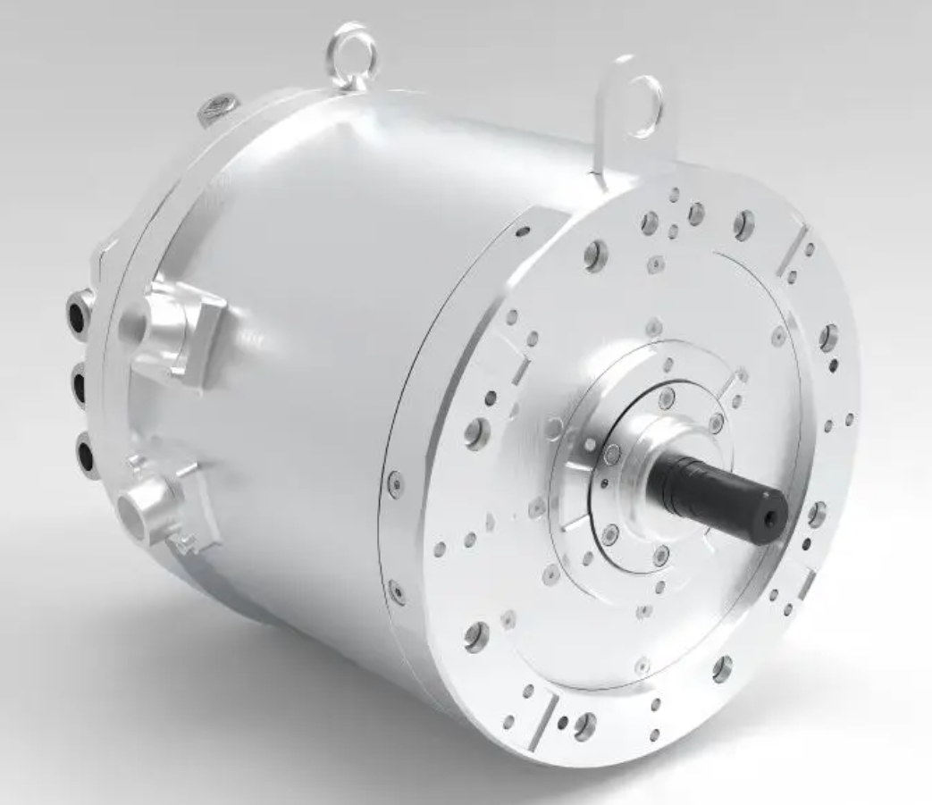
I structure my analysis around four control families that are widely relevant to the PMSM electric motor in electric vehicles: vector control, direct torque control, model predictive control, and intelligent control. I also examine how these methods can be integrated with observers, efficiency optimization, flux weakening, and thermal constraints. Throughout, I use tables and formulas to summarize the relationships that I consider most useful for design and calibration.
Operating Principle and Mathematical Foundation of the PMSM Electric Motor
I begin with the energy-conversion chain of the PMSM electric motor. Three-phase alternating current enters the stator windings, creates a rotating magnetomotive force, and establishes a rotating stator field. This field interacts with the permanent magnet rotor field. The resulting electromagnetic torque drives the rotor, and the mechanical output is delivered to the drivetrain. In my notation, the electrical angular speed and mechanical angular speed are related by the pole-pair number:
$$ \omega_e = p \omega_m $$
where \( \omega_e \) is the electrical angular speed, \( \omega_m \) is the mechanical angular speed, and \( p \) is the number of pole pairs. The mechanical speed in revolutions per minute can be written as:
$$ n_m = \frac{60 \omega_m}{2\pi} $$
For a PMSM electric motor, the stator voltage equations in the rotor reference frame are essential for control design. I write them as:
$$ v_d = R_s i_d + L_d \frac{di_d}{dt} – \omega_e L_q i_q $$
$$ v_q = R_s i_q + L_q \frac{di_q}{dt} + \omega_e (L_d i_d + \psi_f) $$
Here, \( v_d \) and \( v_q \) are the d-axis and q-axis stator voltages, \( i_d \) and \( i_q \) are the corresponding currents, \( R_s \) is the stator resistance, \( L_d \) and \( L_q \) are the d-axis and q-axis inductances, and \( \psi_f \) is the permanent magnet flux linkage. The flux linkages are:
$$ \psi_d = L_d i_d + \psi_f $$
$$ \psi_q = L_q i_q $$
The electromagnetic torque of the PMSM electric motor can be expressed as:
$$ T_e = \frac{3}{2} p \left[ \psi_f i_q + (L_d – L_q) i_d i_q \right] $$
For a surface-mounted PMSM electric motor, where \( L_d \approx L_q \), the reluctance term vanishes and the torque becomes proportional to the q-axis current:
$$ T_e = \frac{3}{2} p \psi_f i_q $$
For an interior PMSM electric motor, \( L_d \neq L_q \), and the reluctance torque component becomes useful for efficiency improvement and flux weakening. The mechanical dynamics are:
$$ J \frac{d\omega_m}{dt} = T_e – T_L – B \omega_m $$
where \( J \) is the rotor and load inertia, \( T_L \) is the load torque, and \( B \) is the viscous friction coefficient. The copper loss, iron loss, and mechanical output power can be summarized as:
$$ P_{cu} = \frac{3}{2} R_s (i_d^2 + i_q^2) $$
$$ P_{mech} = T_e \omega_m $$
$$ \eta = \frac{P_{out}}{P_{in}} = \frac{P_{mech}}{P_{mech} + P_{cu} + P_{fe} + P_{mech,loss}} $$
I find it useful to keep a compact symbol table when tuning a PMSM electric motor controller.
| Symbol | Meaning | Typical Control Role |
|---|---|---|
| \( R_s \) | Stator resistance | Copper-loss estimate and feedforward decoupling |
| \( L_d, L_q \) | d-axis and q-axis inductances | Current-loop plant model and MTPA |
| \( \psi_f \) | Permanent magnet flux linkage | Torque constant and back-EMF estimation |
| \( p \) | Pole pairs | Electrical and mechanical speed conversion |
| \( i_d, i_q \) | d-axis and q-axis currents | Flux and torque control |
| \( T_e, T_L \) | Electromagnetic and load torque | Dynamic response and speed regulation |
| \( \omega_e, \omega_m \) | Electrical and mechanical speed | Field orientation and flux weakening |
In my experience, the PMSM electric motor model is accurate enough for high-performance control only when the parameters are allowed to vary. Resistance changes with temperature, permanent magnet flux changes with temperature and aging, and inductance changes with current because of magnetic saturation. Therefore, the control method must either estimate these variations or be robust to them.
Application Advantages of the PMSM Electric Motor in Electric Vehicles
I classify the advantages of the PMSM electric motor in electric vehicles into four areas: range, power performance, reliability, and controllability. These advantages are not independent. A control method that improves efficiency may also affect thermal behavior; a method that improves torque response may increase current ripple and loss. I summarize the main advantages in the following table.
| Advantage | Physical or Control Mechanism | Vehicle-Level Effect | Control Objective |
|---|---|---|---|
| Extended driving range | The PMSM electric motor field is supplied by permanent magnets, so no separate excitation current is required. | Lower copper loss and higher efficiency during frequent starts and speed changes. | Minimize loss over torque-speed operating points. |
| High power density | Compact structure and high torque per ampere. | Higher motor power within limited vehicle space. | Track torque reference with minimal current. |
| Fast torque response | High starting torque and rapid current control. | Better launch, acceleration, and overtaking behavior. | Synchronize current loop and speed loop bandwidth. |
| High reliability | Simple rotor structure and stable permanent magnet field. | Fewer mechanical and electrical failure modes. | Maintain control under parameter drift and faults. |
| Environmental tolerance | Permanent magnet materials can retain performance over a wide temperature range, with proper thermal design. | Stable operation in hot, cold, and humid conditions. | Limit current and temperature within safe bounds. |
| Regenerative braking capability | Controlled negative q-axis current produces braking torque and energy recovery. | Improved energy efficiency in urban driving. | Coordinate braking torque with battery charging limits. |
I have found that the efficiency advantage of the PMSM electric motor is strongest when the control strategy continuously adapts the d-axis and q-axis currents. A fixed \( i_d = 0 \) strategy is simple, but it does not exploit reluctance torque in an interior PMSM electric motor. Conversely, a poorly designed efficiency strategy can reduce dynamic response or push the inverter into overmodulation. Therefore, I treat efficiency as a constrained optimization problem rather than a standalone rule.
Vector Control of the PMSM Electric Motor
Vector control, also called field-oriented control, is the method I most often use as a baseline for the PMSM electric motor. Its central idea is to transform the three-phase stationary variables into a two-axis rotating reference frame. In that frame, the stator current is decomposed into a flux-producing component \( i_d \) and a torque-producing component \( i_q \). I can then control these components independently, which makes the PMSM electric motor behave in a manner similar to a separately excited DC machine.
The Clarke transformation from three-phase currents to the stationary \( \alpha\beta \) frame is:
$$ \begin{bmatrix} i_\alpha \\ i_\beta \end{bmatrix} = \frac{2}{3} \begin{bmatrix} 1 & -\frac{1}{2} & -\frac{1}{2} \\ 0 & \frac{\sqrt{3}}{2} & -\frac{\sqrt{3}}{2} \end{bmatrix} \begin{bmatrix} i_a \\ i_b \\ i_c \end{bmatrix} $$
The Park transformation from the stationary frame to the rotor dq frame is:
$$ \begin{bmatrix} i_d \\ i_q \end{bmatrix} = \begin{bmatrix} \cos\theta_e & \sin\theta_e \\ -\sin\theta_e & \cos\theta_e \end{bmatrix} \begin{bmatrix} i_\alpha \\ i_\beta \end{bmatrix} $$
where \( \theta_e \) is the electrical rotor angle. The inverse Park transformation is:
$$ \begin{bmatrix} i_\alpha \\ i_\beta \end{bmatrix} = \begin{bmatrix} \cos\theta_e & -\sin\theta_e \\ \sin\theta_e & \cos\theta_e \end{bmatrix} \begin{bmatrix} i_d \\ i_q \end{bmatrix} $$
For current regulation, I use proportional-integral controllers with feedforward decoupling. A representative d-axis voltage command is:
$$ v_d^* = R_s i_d^* – \omega_e L_q i_q^* + K_{p,d}(i_d^* – i_d) + K_{i,d} \int (i_d^* – i_d) dt $$
A representative q-axis voltage command is:
$$ v_q^* = R_s i_q^* + \omega_e (L_d i_d^* + \psi_f) + K_{p,q}(i_q^* – i_q) + K_{i,q} \int (i_q^* – i_q) dt $$
The feedforward terms compensate for cross-coupling and back-EMF. Without them, the current loops must fight the coupling, and the achievable bandwidth is lower. I summarize the vector-control structure in the following table.
| Layer | Function | Typical Signal | Design Consideration |
|---|---|---|---|
| Speed loop | Generate torque reference | \( T_e^* \) or \( i_q^* \) | Bandwidth must be below current-loop bandwidth. |
| Current loop | Regulate \( i_d \) and \( i_q \) | \( v_d^*, v_q^* \) | Gain scheduling for saturation and temperature. |
| Coordinate transform | Convert measured currents and voltages | \( i_\alpha, i_\beta, i_d, i_q \) | Accurate rotor angle is critical. |
| Modulation | Generate inverter switching | SVPWM duty cycles | Limit voltage to linear modulation range. |
| Reference generation | Define \( i_d^* \) and \( i_q^* \) | MTPA or flux-weakening table | Balance torque, efficiency, and voltage limit. |
For an interior PMSM electric motor, the maximum-torque-per-ampere condition is obtained by minimizing stator current amplitude for a given torque. A common expression for the d-axis current is:
$$ i_d = \frac{\psi_f}{2(L_q – L_d)} – \sqrt{ \frac{\psi_f^2}{4(L_q – L_d)^2} + i_q^2 } $$
For a surface-mounted PMSM electric motor, I often use \( i_d^* = 0 \) because the reluctance torque is negligible. For an interior PMSM electric motor, I use a look-up table or an online solver to find the MTPA point. In my view, vector control remains the most practical foundation because it provides a clear separation between flux and torque, and because it supports field weakening, MTPA, and sensorless operation.
I also note the limitations of vector control. The method depends on rotor angle and parameter accuracy. If \( \psi_f \), \( L_d \), or \( L_q \) are incorrect, the torque estimate and decoupling terms become biased. Temperature drift in \( R_s \) also affects the voltage feedforward. In addition, coordinate transformations and multiple PI loops increase computational load compared with simple scalar control, though modern digital signal processors handle this easily.
Direct Torque Control of the PMSM Electric Motor
Direct torque control is the second family I consider for the PMSM electric motor. Unlike vector control, direct torque control works directly in the stator reference frame. It estimates stator flux and electromagnetic torque, compares them with references through hysteresis controllers, and selects an inverter voltage vector from a switching table. The method is attractive because it does not require a modulator in its classical form and because it can produce very fast torque response.
The stator flux estimate is:
$$ \psi_s = \int (v_s – R_s i_s) dt $$
In the stationary \( \alpha\beta \) frame, the components are:
$$ \psi_{s\alpha} = \int (v_{s\alpha} – R_s i_{s\alpha}) dt $$
$$ \psi_{s\beta} = \int (v_{s\beta} – R_s i_{s\beta}) dt $$
The stator flux magnitude is:
$$ |\psi_s| = \sqrt{\psi_{s\alpha}^2 + \psi_{s\beta}^2} $$
The electromagnetic torque can be estimated as:
$$ T_e = \frac{3}{2} p (\psi_{s\alpha} i_{s\beta} – \psi_{s\beta} i_{s\alpha}) $$
I define the torque error and flux error as:
$$ \Delta T_e = T_e^* – T_e $$
$$ \Delta \psi_s = \psi_s^* – |\psi_s| $$
Hysteresis controllers then produce discrete outputs. For example, a simple three-level torque hysteresis controller can be written as:
$$ H_T = \begin{cases} 1, & \Delta T_e > +h_T \\ 0, & -h_T \le \Delta T_e \le +h_T \\ -1, & \Delta T_e < -h_T \end{cases} $$
Similarly, the flux hysteresis controller can be:
$$ H_\psi = \begin{cases} 1, & \Delta \psi_s > +h_\psi \\ 0, & -h_\psi \le \Delta \psi_s \le +h_\psi \\ -1, & \Delta \psi_s < -h_\psi \end{cases} $$
The classical direct torque control switching table for a two-level inverter can be summarized as follows. The exact table depends on the sector definition and the desired convention, but the principle is that the selected voltage vector must increase or decrease flux and torque according to the hysteresis outputs.
| Sector | \( H_\psi = 1, H_T = 1 \) | \( H_\psi = 1, H_T = 0 \) | \( H_\psi = 1, H_T = -1 \) | \( H_\psi = 0, H_T = 1 \) | \( H_\psi = 0, H_T = 0 \) | \( H_\psi = 0, H_T = -1 \) |
|---|---|---|---|---|---|---|
| 1 | \( V_2 \) | \( V_7 \) | \( V_6 \) | \( V_3 \) | \( V_0 \) | \( V_5 \) |
| 2 | \( V_3 \) | \( V_0 \) | \( V_1 \) | \( V_4 \) | \( V_7 \) | \( V_6 \) |
| 3 | \( V_4 \) | \( V_7 \) | \( V_2 \) | \( V_5 \) | \( V_0 \) | \( V_1 \) |
| 4 | \( V_5 \) | \( V_0 \) | \( V_3 \) | \( V_6 \) | \( V_7 \) | \( V_2 \) |
| 5 | \( V_6 \) | \( V_7 \) | \( V_4 \) | \( V_1 \) | \( V_0 \) | \( V_3 \) |
| 6 | \( V_1 \) | \( V_0 \) | \( V_5 \) | \( V_2 \) | \( V_7 \) | \( V_4 \) |
I find direct torque control appealing for the PMSM electric motor in electric vehicles because it responds quickly to torque demand. When the driver requests a rapid increase in torque, direct torque control can change the voltage vector immediately. It is also less dependent on rotor angle than vector control in its basic form, which can be an advantage when the position sensor is noisy or when sensorless estimation is imperfect. However, the classical method produces torque and flux ripple because it selects from a finite set of voltage vectors and because the switching frequency is variable. This ripple can create acoustic noise and additional loss.
To reduce ripple, I often use space-vector modulation with direct torque control. The reference voltage vector can be synthesized as:
$$ V_{ref} = \frac{2}{3} \left( v_a + a v_b + a^2 v_c \right) $$
where:
$$ a = e^{j 2\pi/3} $$
In SVM-DTC, the hysteresis controllers are replaced or augmented by a predictive or PI-based controller that calculates the required voltage vector, and the modulator applies it with fixed switching frequency. This hybrid approach keeps the fast torque response of direct torque control while reducing ripple. I compare vector control and direct torque control in the table below.
| Criterion | Vector Control | Direct Torque Control |
|---|---|---|
| Reference frame | Rotor dq frame | Stator \( \alpha\beta \) frame |
| Current control | Explicit \( i_d \), \( i_q \) regulation | Implicit through torque and flux |
| Torque response | Fast, limited by current-loop bandwidth | Very fast, limited by switching selection |
| Torque ripple | Low with SVPWM | Higher in classical form |
| Parameter sensitivity | Moderate to high | Lower in classical form |
| Switching frequency | Fixed with PWM | Variable in classical form |
| Computational load | Moderate | Low to moderate |
| Typical PMSM electric motor use | High-performance traction and industrial drives | Fast torque applications and robust drives |
Model Predictive Control of the PMSM Electric Motor
Model predictive control is the third family I examine for the PMSM electric motor. In my view, it is attractive because it can handle multiple objectives and constraints directly. Instead of tuning separate loops for torque, flux, current, and voltage, I define a cost function that expresses what the PMSM electric motor should do over a prediction horizon. The controller then solves an optimization problem at each sampling instant.
I start with a discrete-time state-space model. Let the state vector be:
$$ x_k = \begin{bmatrix} i_d(k) \\ i_q(k) \\ \omega_m(k) \end{bmatrix} $$
Let the input vector be:
$$ u_k = \begin{bmatrix} v_d(k) \\ v_q(k) \end{bmatrix} $$
A simplified discrete model for the PMSM electric motor is:
$$ i_d^{k+1} = i_d^k + \frac{T_s}{L_d} \left( v_d^k – R_s i_d^k + \omega_e^k L_q i_q^k \right) $$
$$ i_q^{k+1} = i_q^k + \frac{T_s}{L_q} \left( v_q^k – R_s i_q^k – \omega_e^k L_d i_d^k – \omega_e^k \psi_f \right) $$
$$ \omega_m^{k+1} = \omega_m^k + \frac{T_s}{J} \left( T_e^k – T_L^k – B \omega_m^k \right) $$
The general state-space form is:
$$ x_{k+1} = A x_k + B u_k + d_k $$
where \( d_k \) represents disturbances and modeling errors. For finite-control-set model predictive control, the input is not a continuous voltage but one of the eight switching states of a two-level inverter. I evaluate the predicted response for each candidate voltage vector and choose the one that minimizes the cost function. A representative cost function is:
$$ g = \sum_{j=1}^{N_p} \left[ \lambda_T (T_e^* – T_e^{k+j})^2 + \lambda_\psi (\psi_s^* – \psi_s^{k+j})^2 + \lambda_d (i_d^* – i_d^{k+j})^2 + \lambda_q (i_q^* – i_q^{k+j})^2 \right] + \sum_{j=0}^{N_c-1} \lambda_u \Delta u_{k+j}^2 $$
Here, \( N_p \) is the prediction horizon, \( N_c \) is the control horizon, and \( \lambda_T \), \( \lambda_\psi \), \( \lambda_d \), \( \lambda_q \), and \( \lambda_u \) are weighting factors. I also include constraints such as:
$$ |i_s| = \sqrt{i_d^2 + i_q^2} \le I_{max} $$
$$ |v_s| = \sqrt{v_d^2 + v_q^2} \le \frac{V_{dc}}{\sqrt{3}} $$
$$ |T_e| \le T_{max} $$
$$ |\omega_m| \le \omega_{max} $$
$$ T_{pm} \le T_{pm,max} $$
In my design practice, the weighting factors are not arbitrary. I tune them by considering the relative importance of torque tracking, flux tracking, current limitation, and switching loss. If \( \lambda_u \) is too small, the PMSM electric motor may respond quickly but with high switching loss and acoustic noise. If \( \lambda_T \) is too large, the controller may push current close to the limit and reduce efficiency. I summarize the main variants of model predictive control in the following table.
| Variant | Decision Variable | Advantage | Challenge |
|---|---|---|---|
| Finite-control-set MPC | Inverter switching state | Direct handling of discrete inputs | High torque ripple and variable switching frequency |
| Continuous-control-set MPC | Voltage vector | Smooth voltage and fixed switching frequency with modulator | Requires modulation and more computation |
| MPC with current constraints | \( i_d, i_q \) references | Protects inverter and motor | Constraint handling increases computation |
| MPC with efficiency cost | Loss terms | Improves range | Loss model must be accurate |
| Long-horizon MPC | Multiple future steps | Better global behavior | Computation grows rapidly |
I have found that model predictive control is especially useful for the PMSM electric motor when the operating conditions change quickly. For example, during emergency overtaking, the controller can prioritize torque response and temporarily relax efficiency weighting. During steady cruising, it can shift weighting toward loss minimization and current ripple reduction. The main drawback is computational burden. I address this by using a short prediction horizon, a fast predictive model, explicit constraints, and precomputed lookup tables for common operating regions.
Intelligent Control of the PMSM Electric Motor
Intelligent control is the fourth family I consider for the PMSM electric motor. I use the term to include fuzzy control, neural network control, and hybrid neuro-fuzzy control. These methods are useful when the plant is nonlinear, when parameters vary widely, or when an accurate model is difficult to obtain. In my view, intelligent control should not replace fundamental electromagnetic control. Instead, it should augment the current loop, speed loop, or reference generator of the PMSM electric motor.
Fuzzy control maps linguistic rules into control actions. For a speed-controlled PMSM electric motor, I define the speed error and error change as:
$$ e(k) = \omega_m^*(k) – \omega_m(k) $$
$$ \Delta e(k) = e(k) – e(k-1) $$
The fuzzy controller output can be represented as:
$$ u(k) = \frac{\sum_{i=1}^{N} \mu_i(e,\Delta e) u_i}{\sum_{i=1}^{N} \mu_i(e,\Delta e)} $$
where \( \mu_i \) are membership degrees and \( u_i \) are rule consequents. A typical rule is: if speed error is positive large and error change is positive small, then increase torque command. I have used fuzzy logic to shape the speed response of a PMSM electric motor so that it is fast without overshoot. The main difficulty is rule definition. Poorly defined membership functions can cause oscillation or sluggish response.
Neural network control uses learning and approximation. A multilayer perceptron can be written as:
$$ y = f_2 \left( W_2 f_1(W_1 x + b_1) + b_2 \right) $$
For the PMSM electric motor, the input vector \( x \) can include speed reference, actual speed, d-axis current, q-axis current, DC-link voltage, and temperature. The output \( y \) can be a voltage command, a current reference, or a gain correction. Training usually minimizes a cost such as:
$$ J = \frac{1}{2} \sum_{k=1}^{N} \left( y^*(k) – y(k) \right)^2 $$
Gradient descent updates the weights as:
$$ W^{(t+1)} = W^{(t)} – \eta \frac{\partial J}{\partial W} $$
where \( \eta \) is the learning rate. I have observed that neural network control can adapt to nonlinear torque production in an interior PMSM electric motor, but it requires data covering a wide operating range. If training data are limited, the controller may behave poorly outside the training domain.
Neuro-fuzzy control combines the interpretability of fuzzy rules with the learning ability of neural networks. A common normalized output form is:
$$ \hat{y} = \frac{\sum_{i=1}^{R} \bar{w}_i f_i}{\sum_{i=1}^{R} \bar{w}_i} $$
where \( \bar{w}_i \) are normalized firing strengths. In my view, neuro-fuzzy control is promising for the PMSM electric motor because it can adapt membership functions and consequents online. However, it increases calibration complexity and requires safety supervision. I compare intelligent control methods in the table below.
| Method | Core Mechanism | Strength for PMSM Electric Motor | Limitation |
|---|---|---|---|
| Fuzzy control | Linguistic rules and membership functions | Robust to parameter variation and external disturbance | Rule design depends on experience |
| Neural network control | Learning nonlinear mappings | Adapts to complex nonlinear behavior | Needs large data sets and careful validation |
| Neuro-fuzzy control | Fuzzy structure with learning | Combines interpretability and adaptation | High design and tuning complexity |
| Reinforcement-learning-assisted control | Trial-and-error policy optimization | Can optimize long-term efficiency and response | Safety and real-time constraints are difficult |
| Expert-system supervision | Rule-based fault and mode management | Improves reliability and diagnostics | Knowledge base must be maintained |
Observer Design and Sensorless Operation for the PMSM Electric Motor
I cannot discuss high-efficiency control of the PMSM electric motor without addressing rotor position and speed estimation. Vector control and model predictive control both require accurate rotor angle, and direct torque control benefits from accurate flux estimation. In many electric vehicle drives, a resolver or encoder is used, but sensorless operation reduces cost and improves fault tolerance. I often use a back-EMF observer for medium and high speeds. The stationary-frame back-EMF components can be estimated as:
$$ \hat{e}_\alpha = v_\alpha – R_s i_\alpha – L_s \frac{di_\alpha}{dt} $$
$$ \hat{e}_\beta = v_\beta – R_s i_\beta – L_s \frac{di_\beta}{dt} $$
The rotor angle can then be estimated from:
$$ \hat{\theta}_e = \tan^{-1} \left( -\frac{\hat{e}_\alpha}{\hat{e}_\beta} \right) $$
For low-speed operation, back-EMF is small, so I use high-frequency signal injection or a saliency-based method. For a Kalman filter observer, I write the prediction and update equations as:
$$ \hat{x}_{k|k-1} = F \hat{x}_{k-1|k-1} + B u_{k-1} $$
$$ P_{k|k-1} = F P_{k-1|k-1} F^T + Q $$
$$ K_k = P_{k|k-1} H^T \left( H P_{k|k-1} H^T + R \right)^{-1} $$
$$ \hat{x}_{k|k} = \hat{x}_{k|k-1} + K_k \left( z_k – H \hat{x}_{k|k-1} \right) $$
$$ P_{k|k} = \left( I – K_k H \right) P_{k|k-1} $$
I use \( Q \) and \( R \) to trade off model confidence against measurement confidence. In my view, the observer is not a separate add-on. It is part of the control architecture, and its bandwidth must be coordinated with the current and speed loops. If the observer is too slow, the PMSM electric motor loses field orientation. If it is too fast, it amplifies noise and causes current ripple.
Efficiency Optimization and Flux Weakening of the PMSM Electric Motor
Efficiency optimization is where I connect control theory to vehicle range. The total loss of the PMSM electric motor includes copper loss, iron loss, inverter loss, windage, and friction. A simplified loss function is:
$$ P_{loss} = P_{cu} + P_{fe} + P_{inv} + P_{mech} $$
The copper loss is:
$$ P_{cu} = \frac{3}{2} R_s (i_d^2 + i_q^2) $$
Iron loss can be approximated as a function of electrical frequency and flux:
$$ P_{fe} = k_h \omega_e \psi_s^2 + k_e \omega_e^2 \psi_s^2 $$
I then solve an optimization problem:
$$ \min_{i_d, i_q} P_{loss} $$
subject to the torque constraint:
$$ T_e^* = \frac{3}{2} p \left[ \psi_f i_q + (L_d – L_q) i_d i_q \right] $$
and current and voltage constraints:
$$ i_d^2 + i_q^2 \le I_{max}^2 $$
$$ v_d^2 + v_q^2 \le V_{max}^2 $$
For a given torque and speed, I can find the current pair that minimizes loss. In practice, I use a lookup table generated offline and then corrected online for temperature and DC-link voltage. The PMSM electric motor operating point can be divided into three regions:
| Region | Speed Range | Current Strategy | Main Objective |
|---|---|---|---|
| Constant-torque region | Below base speed | MTPA or \( i_d = 0 \) for surface PMSM electric motor | Maximum torque per ampere |
| Constant-power region | Above base speed | Negative \( i_d \) for flux weakening | Maintain torque under voltage limit |
| Deep flux-weakening region | Near maximum speed | Strong negative \( i_d \), reduced \( i_q \) | Prevent voltage saturation and protect inverter |
A commonly used flux-weakening current expression is:
$$ i_d^{fw} = -\frac{\psi_f}{L_d} + \sqrt{ \left( \frac{V_{max}}{\omega_e L_d} \right)^2 – \left( i_q \frac{L_q}{L_d} \right)^2 } $$
I must also respect the voltage limit ellipse:
$$ (L_d i_d + \psi_f)^2 + (L_q i_q)^2 \le \left( \frac{V_{max}}{\omega_e} \right)^2 $$
and the current limit circle:
$$ i_d^2 + i_q^2 \le I_{max}^2 $$
In my view, flux weakening is one of the most important control functions for the PMSM electric motor in electric vehicles. Without it, the motor cannot reach high speed efficiently. With poorly coordinated flux weakening, the motor may draw excessive current, overheat, or lose torque control. I therefore integrate flux weakening with the current reference generator and the inverter voltage margin.
Thermal Management and Reliability Control of the PMSM Electric Motor
I treat thermal behavior as a first-class constraint in high-efficiency control of the PMSM electric motor. The stator winding temperature and permanent magnet temperature affect resistance, flux linkage, and insulation life. A simplified thermal model is:
$$ C_{th} \frac{dT}{dt} = P_{loss} – \frac{T – T_{amb}}{R_{th}} $$
where \( C_{th} \) is thermal capacitance, \( R_{th} \) is thermal resistance, \( T \) is the component temperature, and \( T_{amb} \) is ambient temperature. I use this model to derate current when temperature rises. A simple derating rule is:
$$ I_{max}(T) = \begin{cases} I_{rated}, & T \le T_{low} \\ I_{rated} \frac{T_{max} – T}{T_{max} – T_{low}}, & T_{low} < T < T_{max} \\ 0, & T \ge T_{max} \end{cases} $$
For the PMSM electric motor, magnet temperature is especially important because high temperature reduces \( \psi_f \) and therefore reduces torque per ampere. If the controller does not compensate, the driver may demand more current for the same torque, which increases loss and temperature further. I therefore use temperature-dependent torque maps and current limits. I also monitor inverter temperature, DC-link voltage, phase current, and speed to detect faults.
| Reliability Function | Monitored Signal | Control Action | Benefit for PMSM Electric Motor |
|---|---|---|---|
| Overcurrent protection | \( i_a, i_b, i_c \) or \( i_d, i_q \) | Limit current reference and disable PWM | Protects windings and inverter |
| Overvoltage protection | DC-link voltage | Activate braking chopper or reduce regenerative torque | Protects capacitors and switches |
| Overtemperature protection | Stator and magnet temperature | Derate torque and current | Prevents demagnetization and insulation damage |
| Position fault detection | Resolver or encoder signals | Switch to sensorless mode or limp-home mode | Maintains controllability |
| Parameter drift compensation | Temperature and current | Update \( R_s \), \( \psi_f \), \( L_d \), \( L_q \) | Preserves torque accuracy and efficiency |
Integrated Control Architecture for the PMSM Electric Motor
In my design approach, I do not choose a single control method in isolation. I build an integrated architecture for the PMSM electric motor. The outer layer manages vehicle torque demand, battery limits, thermal limits, and driving mode. The middle layer generates optimal current references using MTPA, flux weakening, and loss minimization. The inner layer regulates current with vector control, direct torque control, or model predictive control. The observer layer estimates rotor angle, speed, and disturbances. The supervision layer monitors faults and enforces constraints.
A representative integrated control law can be written as:
$$ u^* = \arg \min_{u \in U} \left[ J_{track}(x,u) + J_{loss}(x,u) + J_{smooth}(u) \right] $$
subject to:
$$ x_{k+1} = f(x_k, u_k) $$
$$ g(x_k, u_k) \le 0 $$
where \( J_{track} \) penalizes torque and speed error, \( J_{loss} \) penalizes copper and iron loss, and \( J_{smooth} \) penalizes switching or current ripple. I have found that this formulation unifies the strengths of the four control families. Vector control provides reliable current regulation. Direct torque control provides fast torque transients. Model predictive control provides constraint handling. Intelligent control provides adaptation and nonlinear compensation.
| Layer | Function | Preferred Method | Key Output |
|---|---|---|---|
| Vehicle supervisor | Torque demand and energy management | Rule-based and optimization | \( T_e^* \) and operating mode |
| Reference generator | MTPA, flux weakening, loss minimization | Lookup table and online optimization | \( i_d^*, i_q^* \) |
| Current controller | Fast current tracking | Vector control or MPC | \( v_d^*, v_q^* \) |
| Torque transient controller | Fast torque response | Direct torque control or MPC | Voltage vector or switching state |
| Observer | Position, speed, and disturbance estimation | Back-EMF observer, Kalman filter | \( \hat{\theta}_e, \hat{\omega}_m \) |
| Supervisor | Fault detection and thermal protection | Rule-based and intelligent diagnostics | Derating and fault flags |
Comparative Assessment of Control Methods for the PMSM Electric Motor
I now compare the four control families across the criteria that matter most for electric vehicles. I use a qualitative scale from low to high. The comparison is not absolute because each method can be modified and hybridized. Nevertheless, it helps me select a control strategy for a given PMSM electric motor application.
| Criterion | Vector Control | Direct Torque Control | Model Predictive Control | Intelligent Control |
|---|---|---|---|---|
| Steady-state efficiency | High with MTPA and loss model | Moderate to high | High with loss-aware cost function | High if trained well |
| Torque response | High | Very high | Very high | Moderate to high |
| Torque ripple | Low | Moderate to high | Low to moderate with long horizon | Depends on design |
| Parameter sensitivity | Moderate to high | Low to moderate | Moderate to high | Low with adaptation |
| Computational cost | Moderate | Low | High | Moderate to high |
| Constraint handling | Indirect | Limited | Direct | Indirect |
| Calibration effort | Moderate | Moderate | High | High |
| Robustness | Moderate | High | Moderate to high | High with proper training |
| Best use in PMSM electric motor | Baseline traction control | Fast transient and robust drives | Multi-objective traction control | Adaptive and fault-tolerant control |
From my perspective, vector control is the most mature and predictable choice for the PMSM electric motor. Direct torque control is valuable when the torque transient is the dominant requirement. Model predictive control is valuable when multiple constraints must be respected explicitly. Intelligent control is valuable when the operating environment is highly uncertain or when the motor is used across a very wide range of temperatures and loads. In a production electric vehicle, I would likely use vector control as the inner current loop, model predictive control or direct torque control for transient coordination, and intelligent supervision for adaptation and diagnostics.
Practical Tuning Rules I Apply to the PMSM Electric Motor
I close my analysis with practical rules that I use when tuning a high-efficiency PMSM electric motor. These rules are not a substitute for simulation and testing, but they help me organize the calibration process.
| Tuning Area | Rule I Apply | Reason |
|---|---|---|
| Current-loop bandwidth | Set at least five to ten times the speed-loop bandwidth. | Ensures the PMSM electric motor follows current references without interaction. |
| Speed-loop bandwidth | Set below the mechanical resonance and below the observer bandwidth. | Avoids oscillation and noise amplification. |
| Feedforward decoupling | Use measured speed and estimated flux linkage. | Reduces cross-coupling and improves transient response. |
| MTPA table | Generate from electromagnetic parameters and validate with efficiency maps. | Ensures the PMSM electric motor uses minimum current for torque. |
| Flux weakening | Activate before voltage saturation, not after. | Prevents current spikes and loss of control at high speed. |
| MPC weighting | Tune torque weight first, then current limit, then switching smoothness. | Keeps the cost function physically meaningful. |
| Intelligent controller | Use only inside validated operating bounds with a fallback controller. | Protects the PMSM electric motor from unsafe learned actions. |
| Thermal derating | Derate gradually and compensate \( R_s \) and \( \psi_f \) with temperature. | Maintains torque accuracy and protects magnets. |
I also recommend that the control software maintain a clear separation between torque-producing current and flux-producing current. This separation makes diagnostics easier. If the PMSM electric motor produces less torque than expected, I can check whether \( i_q \) is limited, whether \( \psi_f \) has dropped with temperature, or whether the voltage limit is forcing a flux-weakening current. If efficiency is lower than expected, I can examine copper loss, iron loss, and inverter switching loss separately.
Conclusion
In my assessment, high-efficiency control of the PMSM electric motor in electric vehicles is a layered and multi-objective discipline. The PMSM electric motor offers high power density, high efficiency, fast torque response, and strong reliability, but these benefits are realized only when the control method manages current, flux, voltage, temperature, and parameter variation together. Vector control provides a robust foundation through field orientation and independent control of \( i_d \) and \( i_q \). Direct torque control provides very fast torque response and strong robustness. Model predictive control provides direct constraint handling and multi-objective optimization. Intelligent control provides adaptation and nonlinear compensation when the plant is uncertain or highly variable.
I conclude that the most effective strategy is not to select one method exclusively, but to integrate them according to the operating mode of the PMSM electric motor. In low-speed launch, I prioritize torque response and current limiting. In steady cruising, I prioritize loss minimization and smooth switching. In high-speed operation, I prioritize flux weakening and voltage margin. In fault conditions, I prioritize derating, observer fallback, and safe shutdown. By combining mathematical models, optimization, observers, and intelligent supervision, I can help ensure that the PMSM electric motor delivers stable, reliable, and efficient performance throughout the electric vehicle operating range.