
I study a compact, high-accuracy current-measurement solution for the electric vehicle battery pack, where the available installation space is narrow, the busbar is usually rectangular, and the measured current can reach very high values. In an electric vehicle battery pack, the battery management system relies on current data to estimate state of charge, state of health, and thermal risk. Any large drift or nonlinearity in the current sensor can propagate into balancing errors, thermal-management failures, and safety warnings. Therefore, I focus on a coreless Hall array current sensor that avoids magnetic saturation and hysteresis while remaining lightweight, low cost, and suitable for the electric vehicle battery pack.
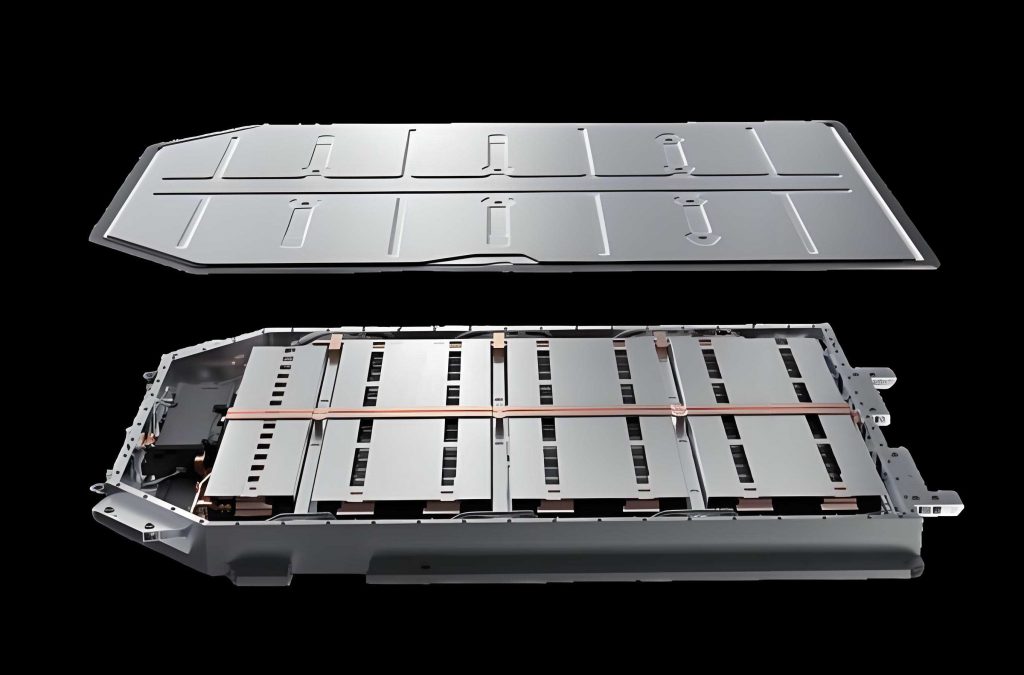
My design is motivated by the fact that conventional current sensors have difficulty simultaneously satisfying the high-current, high-accuracy, low-volume, and low-mass requirements of an electric vehicle battery pack. A shunt is contact-based and introduces insertion loss and insulation complexity. A fluxgate sensor can be accurate but is sensitive to saturation and DC bias, and it is often bulky. A closed-loop Hall sensor uses a magnetic core and compensation winding, which increases mass, volume, and power consumption. For the electric vehicle battery pack, a coreless Hall array is attractive because it reconstructs the current from magnetic field samples around the conductor.
1. Current Measurement Context for Electric Vehicle Battery Packs
I compare the main current-sensing families for the electric vehicle battery pack in Table 1. The comparison shows why I select a Hall array rather than a shunt, fluxgate, or closed-loop Hall sensor. The electric vehicle battery pack demands galvanic isolation, wide dynamic range, low mass, and tolerance to vibration. A coreless Hall array can meet these requirements if its eccentricity and tilt errors are controlled.
| Method | Principle | Contact with Busbar | Magnetic Core | Saturation Risk | Typical Mass and Volume | Suitability for Electric Vehicle Battery Pack |
|---|---|---|---|---|---|---|
| Shunt | Ohm’s law across a sampling resistor | Yes | No | No | Moderate to high | Limited by insertion loss and isolation design |
| Fluxgate | Nonlinear magnetic permeability of a soft core | No | Yes | Yes | High | Accurate but bulky and sensitive to DC bias |
| Open-loop Hall | Hall voltage in an air gap | No | Yes | Yes | Moderate | Low cost but temperature drift remains |
| Closed-loop Hall | Magnetic balance with compensation winding | No | Yes | Reduced | High | Good linearity but high power and volume |
| Coreless Hall array | Ampere-loop reconstruction from multiple Hall elements | No | No | No | Low | Best fit for a narrow electric vehicle battery pack |
In an electric vehicle battery pack, the busbar is often rectangular because a rectangular cross section provides better heat dissipation, lower cost, and easier assembly than a round conductor. However, a circular Hall array around a rectangular busbar wastes space and places some Hall elements far from the conductor. I therefore adopt an elliptical Hall array. The elliptical shape follows the magnetic field distribution around a rectangular busbar more closely and reduces the installation footprint inside the electric vehicle battery pack.
2. Hall Effect and Array Reconstruction
I begin with the Hall effect. When a current-carrying conductor is placed in a magnetic field perpendicular to the current, charge carriers are deflected by the Lorentz force. A transverse electric field is built until the electric force balances the Lorentz force. The resulting Hall voltage is proportional to the magnetic flux density. For a thin Hall plate, the Hall voltage is
$$V_H = K_H B,$$
where \(V_H\) is the Hall voltage, \(K_H\) is the Hall sensitivity, and \(B\) is the magnetic flux density. In a practical Hall integrated circuit, signal amplification, offset cancellation, and temperature compensation may be included, so the output is a conditioned voltage or digital word.
For an open-loop Hall current sensor with a magnetic core and an air gap, the air-gap flux density can be approximated as
$$B_0 \approx \frac{\mu_0 N I}{l_0},$$
where \(\mu_0\) is the vacuum permeability, \(N\) is the number of conductor turns through the core, \(I\) is the primary current, and \(l_0\) is the effective air-gap length. The Hall voltage then becomes
$$V_H \approx K_H \frac{\mu_0 N I}{l_0}.$$
Although this structure is simple, the core introduces saturation, hysteresis, and additional mass. For the electric vehicle battery pack, a coreless array avoids these issues. The array principle is based on Ampere’s circuital law:
$$\oint \mathbf{H} \cdot d\mathbf{l} = I.$$
I place \(N\) Hall elements on a closed elliptical path around the rectangular busbar. The discrete approximation of the line integral is
$$I_{\text{calc}} = \sum_{i=1}^{N} H_{i,\text{MFS}} \Delta s_i,$$
where \(H_{i,\text{MFS}}\) is the magnetic field component along the sensitive axis of the \(i\)-th Hall element and \(\Delta s_i\) is the length of the \(i\)-th curve segment. If the Hall elements are uniformly spaced by the uniform curve segment length method, then \(\Delta s_i = \Delta s\) for all \(i\), and
$$I_{\text{calc}} = \Delta s \sum_{i=1}^{N} H_{i,\text{MFS}}.$$
The relative current error is
$$\varepsilon = \frac{I_{\text{calc}} – I}{I} \times 100\%.$$
Table 2 compares circular, rectangular, and elliptical arrays for an electric vehicle battery pack. The rectangular array follows the busbar shape but has sharp corners where the magnetic field gradient changes abruptly. The circular array is smooth but large. The elliptical array gives a better compromise for a rectangular busbar in a narrow electric vehicle battery pack.
| Array Shape | Advantages | Disadvantages | Fit for Rectangular Busbar | Fit for Narrow Electric Vehicle Battery Pack |
|---|---|---|---|---|
| Circular | Smooth path, mature theory | Large footprint, low signal-to-noise ratio at far elements | Moderate | Poor |
| Rectangular | Follows busbar profile | Field discontinuities at corners, higher numerical error | Good | Moderate |
| Elliptical | Smaller than circular, smoother than rectangular | Requires careful parameter design | Good | Good |
3. Elliptical Array Parameter Design
I design the elliptical array by using the uniform curve segment length method. I also compare it with a projection method. In the projection method, a circular array is projected onto an ellipse by scaling one axis. This makes the curve segment lengths uneven, and some Hall elements become far apart. In the uniform curve segment length method, the ellipse perimeter is divided into equal arc lengths, so the Hall elements are evenly distributed along the elliptical path. I find that the uniform curve segment length method gives lower current error for the same number of Hall elements.
I define the ellipse with semi-major axis \(a\) and semi-minor axis \(b\). The aspect ratio is
$$AR = \frac{b}{a}.$$
The parametric coordinates of the ellipse are
$$x(\theta) = a \cos\theta, \quad y(\theta) = b \sin\theta.$$
To find equal arc-length positions, I approximate the ellipse by \(K\) discrete points. The arc length from the positive \(X\)-axis to the \(k\)-th point is
$$s(k) = \sum_{n=1}^{k} \sqrt{(x_{n} – x_{n-1})^2 + (y_{n} – y_{n-1})^2}.$$
The total perimeter is \(s(K)\). For \(N\) Hall elements, the segment length is
$$\Delta s = \frac{s(K)}{N}.$$
I introduce an initial offset ratio \(s_{r,0}\) to improve robustness. For \(N\) elements, the offset is
$$s_0 = s_{r,0} s(K).$$
The arc length to the \(i\)-th Hall element is
$$s_i = s_0 + i \Delta s, \quad i = 1,2,\dots,N.$$
The position of the \(i\)-th Hall element is obtained by finding the point on the discrete ellipse whose arc length equals \(s_i\). The sensitive axis is the tangent direction of the ellipse at that point. If the point is parameterized by \(\theta_i\), the tangent vector is
$$\mathbf{t}_i = \frac{1}{\sqrt{a^2 \sin^2\theta_i + b^2 \cos^2\theta_i}} \begin{pmatrix} -a \sin\theta_i \\ b \cos\theta_i \end{pmatrix}.$$
I use a rectangular busbar with a cross section of \(20\,\text{mm} \times 4\,\text{mm}\), which is representative of an electric vehicle battery pack. I set the semi-major axis to \(a = 30\,\text{mm}\) to balance footprint and signal strength. I then compute the current error for different numbers of Hall elements and different aspect ratios. The current error decreases as the number of Hall elements increases, but the improvement becomes small beyond \(N=7\). I also find that \(N=6\) with \(AR=0.33\) and \(N=7\) with \(AR=0.31\) have low theoretical error. Considering cost and robustness, I select \(N=6\) and \(AR=0.33\) for the electric vehicle battery pack sensor.
| Array Parameter | Number of Hall Elements | Aspect Ratio | Semi-Major Axis (mm) | Semi-Minor Axis (mm) | Selection Rationale |
|---|---|---|---|---|---|
| Elliptical A | 6 | 0.33 | 30.0 | 9.9 | Low error, small footprint, low cost |
| Elliptical B | 7 | 0.31 | 30.0 | 9.3 | Lower error but higher cost |
| Circular A | 6 | 1.00 | 30.0 | 30.0 | Large footprint, not compact |
| Circular B | 7 | 1.00 | 30.0 | 30.0 | Large footprint, higher cost |
Table 3 lists the positions and sensitive-axis angles for the selected \(N=6\), \(AR=0.33\) array. The coordinates are in millimeters, and the sensitive-axis angle is the angle between the \(X\)-axis sensitive direction and the \(X\)-axis of the coordinate system.
| Hall Element | Position \(x\) (mm) | Position \(y\) (mm) | Sensitive-Axis Angle (degrees) |
|---|---|---|---|
| 1 | 26.94 | 4.40 | 145.79 |
| 2 | 5.57 | 9.83 | 176.38 |
| 3 | -16.59 | 8.33 | 192.58 |
| 4 | -26.94 | -4.40 | 325.79 |
| 5 | -5.56 | -9.83 | 356.38 |
| 6 | 16.59 | -8.33 | 12.58 |
For the electric vehicle battery pack, I also select Hall elements that satisfy the sensitivity, saturation, and temperature requirements. A two-axis Hall element is sufficient for eccentricity compensation, while a three-axis Hall element is needed when tilt must be estimated in three dimensions. I choose a two-axis Hall IC with a sensitivity around \(130\,\text{mV/mT}\), a supply range of \(3.0\,\text{V}\) to \(5.5\,\text{V}\), and a magnetic range of \(\pm 18\,\text{mT}\). I also use a three-axis Hall IC with a small package, digital output, and a sensitivity around \(10.2\,\text{LSB/mT}\) to support tilt estimation. Table 4 summarizes the key electrical requirements for the electric vehicle battery pack sensor.
| Parameter | Two-Axis Hall Element | Three-Axis Hall Element |
|---|---|---|
| Supply voltage | 3.0 V to 5.5 V | 2.8 V to 3.5 V |
| Typical sensitivity | 130 mV/mT | 10.2 LSB/mT |
| Magnetic range | \(\pm 18\,\text{mT}\) | \(\pm 50\,\text{mT}\) |
| Operating temperature | \(-40^\circ\text{C}\) to \(125^\circ\text{C}\) | \(-40^\circ\text{C}\) to \(125^\circ\text{C}\) |
| Output type | Analog | Digital |
| Role in electric vehicle battery pack | Eccentricity measurement | Eccentricity and tilt measurement |
4. Hardware Architecture
I design the hardware of the electric vehicle battery pack current sensor as a modular system. The main blocks are the Hall array, analog conditioning, analog-to-digital conversion, microcontroller, power supply, and controller area network transceiver. A 12 V supply is converted to 5 V by a DC-DC module. The 5 V rail supplies the Hall elements and analog circuits. A low-dropout regulator converts 5 V to 3.3 V for the microcontroller. Each Hall element output passes through a voltage follower for impedance isolation. The conditioned signals are summed and sampled by the microcontroller. The digital result is sent over a CAN transceiver to the host controller of the electric vehicle battery pack.
| Module | Function | Key Requirement for Electric Vehicle Battery Pack |
|---|---|---|
| Hall array | Magnetic field sampling | Low offset, low temperature drift |
| Voltage follower | Impedance isolation | Low output impedance, low noise |
| Adder | Analog summation | Matched gain, low offset |
| DC-DC converter | 12 V to 5 V | High efficiency, protected output |
| LDO regulator | 5 V to 3.3 V | Low dropout, low noise |
| Microcontroller | ADC, processing, CAN | 12-bit ADC, CAN interface, low power |
| CAN transceiver | Communication | High immunity to electromagnetic interference |
The analog front end is important for the electric vehicle battery pack because the magnetic field around a rectangular busbar is not uniform. I use separate amplification stages for small, medium, and large current ranges. For small currents, I use a three-stage amplifier with a total gain of 100. For medium currents, I use a two-stage amplifier with a total gain of 10. For large currents, I use a single-stage amplifier with a gain of 5. This segmented gain improves resolution without saturating the ADC at high currents. The sampling resistor is \(0.47\,\Omega\), and the ADC resolution is 12 bits with 128 sampling points.
5. Initial Error and Full-Temperature Calibration
I define the initial error as the combined effect of manufacturing tolerances, Hall element offset, gain mismatch, and temperature drift. In an electric vehicle battery pack, the temperature can vary from \(-40^\circ\text{C}\) to \(125^\circ\text{C}\). Therefore, a single room-temperature calibration is not sufficient. I design a full-temperature calibration algorithm that includes room-temperature calibration and high-low temperature calibration.
First, the host reads an 8-bit current message from the sensor. I extract the high nibble and low nibble, convert them to decimal values, and compute the difference:
$$\Delta ADC = DEC_{\text{high}} – DEC_{\text{low}}.$$
The sampling voltage is
$$V_{\text{ADC}} = \frac{\Delta ADC}{K} \times \frac{1}{A} \times V_{\text{min}},$$
where \(K=128\) is the number of sampling points, \(A\) is the gain, and \(V_{\text{min}} = 0.001\,\text{V}\). The output current is
$$I_{\text{output}} = \frac{V_{\text{ADC}}}{R_s},$$
where \(R_s = 0.47\,\Omega\). The current deviation is
$$\Delta I = I_{\text{output}} – I_{\text{input}}.$$
I fit the current measurement \(I_{\text{output}}\) and the current deviation \(\Delta I\) with a first-order linear model:
$$\Delta I_{\text{fit}} = k_i I_{\text{output}} + b_i.$$
The compensated current is
$$I_{\text{mea}} = I_{\text{output}} – \Delta I_{\text{fit}}.$$
The residual deviation is
$$\Delta I_{\text{mea}} = I_{\text{mea}} – I_{\text{input}}.$$
The relative error in per mille is
$$\delta_{\text{rel}} = \frac{\Delta I_{\text{mea}}}{I_{\text{input}}} \times 1000.$$
I use separate fits for small, medium, and large current ranges and for positive and negative directions. Table 5 shows representative fitted slopes and intercepts at room temperature. These coefficients are stored in the sensor and used for real-time compensation.
| Current Range | Direction | Slope \(k_i\) | Intercept \(b_i\) |
|---|---|---|---|
| Small | Positive | -0.00505 | 0.04657 |
| Small | Negative | -0.00508 | -0.04342 |
| Medium | Positive | -0.00367 | 0.06019 |
| Medium | Negative | -0.00395 | -0.10566 |
| Large | Positive | -0.00284 | -1.12625 |
| Large | Negative | -0.00316 | 1.12059 |
For high-low temperature calibration, I test at \(-40^\circ\text{C}\), \(25^\circ\text{C}\), and \(125^\circ\text{C}\). I fit the current deviation at each temperature:
$$\Delta I_{\text{low}} = l_i I_{\text{output}} + c_i,$$
$$\Delta I_{\text{normal}} = k_i I_{\text{output}} + b_i,$$
$$\Delta I_{\text{high}} = h_i I_{\text{output}} + a_i.$$
I define the low-temperature drift coefficient as
$$k_{\text{low}} = \frac{l_i – k_i}{65},$$
because the temperature difference between \(-40^\circ\text{C}\) and \(25^\circ\text{C}\) is \(65^\circ\text{C}\). I define the high-temperature drift coefficient as
$$k_{\text{high}} = \frac{h_i – k_i}{100},$$
because the temperature difference between \(125^\circ\text{C}\) and \(25^\circ\text{C}\) is \(100^\circ\text{C}\). The average drift coefficient per degree is
$$k = \frac{k_{\text{high}} + k_{\text{low}}}{2}.$$
The temperature-compensated deviation is
$$\Delta I_{\text{fit,tem}} = (k_i + k T) I_{\text{output}} + b_i.$$
The final compensated current is
$$I_{\text{mea,tem}} = I_{\text{output}} – \Delta I_{\text{fit,tem}}.$$
I apply this full-temperature calibration to the electric vehicle battery pack sensor. The room-temperature calibration reduces the initial relative error by more than 85%, and the high-low temperature calibration reduces the low-temperature error by about 62% and the high-temperature error by about 43%. The final relative error remains within \(3\permil\) over the full temperature range.
6. Eccentricity and Tilt Error Modeling
In an electric vehicle battery pack, vibration and assembly tolerances can make the rectangular busbar deviate from the center of the elliptical array. This creates eccentricity error. The busbar can also tilt relative to the sensor plane, which creates tilt error. I build a three-dimensional magnetic field model to describe both effects.
I set the ellipse center as the origin. The \(X\)-axis is along the semi-major axis, the \(Y\)-axis is along the semi-minor axis, and the \(Z\)-axis is perpendicular to the sensor plane. The busbar axis intersects the \(XOY\) plane at \(Q(x_p, y_p, 0)\). The angle between the busbar axis and the positive \(Z\)-axis is \(\alpha\). The angle between the projection of the busbar axis on the \(XOY\) plane and the positive \(X\)-axis is \(\beta\). The unit direction vector of the busbar is
$$\mathbf{e}_l = (m, n, p) = (\sin\alpha \cos\beta, \sin\alpha \sin\beta, \cos\alpha).$$
For a point \(P(a,b,0)\) on the sensor plane, the vector from the intersection point to the point is
$$\mathbf{QP} = (a – x_p, b – y_p, 0).$$
The perpendicular distance from the point to the busbar axis is
$$\rho = \|\mathbf{e}_l \times \mathbf{QP}\|.$$
The magnetic field at the point is
$$\mathbf{H} = \frac{I}{2\pi \rho} \mathbf{e}_l \times \mathbf{e}_r,$$
where \(\mathbf{e}_r\) is the unit vector from the busbar axis to the point. For a rectangular conductor, I integrate the contributions of all current filaments over the conductor cross section. The \(X\)-component of the magnetic field is
$$H_x = \frac{I}{2\pi A} \iint_S \frac{p(b-y)}{(p(a-x))^2 + (p(b-y))^2 + (m(a-x)+n(b-y))^2} \, dx\,dy,$$
where \(A\) is the conductor cross-sectional area and \(S\) is the projected cross section on the sensor plane. The \(Y\)-component is
$$H_y = \frac{I}{2\pi A} \iint_S \frac{p(a-x)}{(p(a-x))^2 + (p(b-y))^2 + (m(a-x)+n(b-y))^2} \, dx\,dy.$$
The \(Z\)-component is
$$H_z = \frac{I}{2\pi A} \iint_S \frac{m(a-x) + n(b-y)}{(p(a-x))^2 + (p(b-y))^2 + (m(a-x)+n(b-y))^2} \, dx\,dy.$$
When the busbar is ideal and perpendicular to the sensor plane, \(m=1\), \(n=1\), and \(p=0\). The three-dimensional model then reduces to the two-dimensional model. For eccentricity only, the cross section \(S\) shifts by \(x_p\) and \(y_p\) but keeps its shape. I update the integrals as
$$H_{x,p} = \frac{I}{2\pi A} \iint_S \frac{b-y}{(a-x-x_p)^2 + (b-y-y_p)^2} \, dx\,dy,$$
$$H_{y,p} = \frac{I}{2\pi A} \iint_S \frac{a-x}{(a-x-x_p)^2 + (b-y-y_p)^2} \, dx\,dy.$$
Table 6 compares the allowed eccentricity ranges for four array configurations. The elliptical array has a much smaller footprint, but its \(Y\)-direction tolerance is smaller than that of a circular array. This is acceptable for the electric vehicle battery pack because the busbar orientation is controlled, and the elliptical array is more compact.
| Array | \(-X\) Limit (mm) | \(+X\) Limit (mm) | \(-Y\) Limit (mm) | \(+Y\) Limit (mm) |
|---|---|---|---|---|
| Elliptical \(N=6, AR=0.33\) | -10.5 | 10.5 | -2.1 | 2.1 |
| Elliptical \(N=7, AR=0.31\) | -10.7 | 10.7 | -2.0 | 2.0 |
| Circular \(N=6, AR=1.00\) | -14.9 | 14.9 | -20.9 | 20.9 |
| Circular \(N=7, AR=1.00\) | -14.9 | 14.9 | -20.9 | 20.9 |
I also compare the mass and installation area of different solutions. The coreless elliptical array reduces mass by about 82.9% and installation area by about 72.4% compared with a conventional core-based solution. This is a major advantage for the electric vehicle battery pack, where every millimeter and gram matters.
| Solution | Mass (g) | Installation Area (mm\(^2\)) | Maximum \(X\) Eccentricity Error | Maximum \(Y\) Eccentricity Error |
|---|---|---|---|---|
| Fluxgate current sensor | 69.5 | 3290 | Not applicable | Not applicable |
| Circular Hall array | 15.5 | 2827.4 | \(\leq 17.08\%\) | \(\leq 2.21\%\) |
| Elliptical Hall array in my design | 11.9 | 908.5 | \(\leq 4.73\%\) | \(\leq 0.35\%\) |
7. GWO-BP Error Optimization
The eccentricity and tilt parameters cannot be measured directly from the Hall voltages without a model. I use a neural network to estimate the conductor state from the magnetic field samples. A back-propagation neural network can learn nonlinear relationships, but it is sensitive to initial weights and thresholds and can fall into a local optimum. I therefore use the grey wolf optimizer to optimize the initial weights and thresholds of the BP network. The resulting GWO-BP model estimates the conductor state parameters, which are then used to reconstruct the integral region and improve the current calculation.
The BP network structure I use has 18 input nodes, 12 hidden nodes, and 5 output nodes. The inputs are the \(X\), \(Y\), and \(Z\) magnetic field components from six Hall elements. The outputs are the eccentricity parameters \(x_p\) and \(y_p\) and the tilt parameters \(m\), \(n\), and \(p\).
In the grey wolf optimizer, the position of a wolf is updated by
$$\mathbf{D} = |\mathbf{C} \mathbf{X}_p(t) – \mathbf{X}(t)|,$$
$$\mathbf{X}(t+1) = \mathbf{X}_p(t) – \mathbf{A} \mathbf{D},$$
where \(\mathbf{X}_p\) is the prey position and \(\mathbf{X}\) is the wolf position. The coefficient vectors are
$$\mathbf{A} = 2a \mathbf{r}_1 – a,$$
$$\mathbf{C} = 2 \mathbf{r}_2,$$
where \(\mathbf{r}_1\) and \(\mathbf{r}_2\) are random vectors in \([0,1]\), and \(a\) decreases linearly from 2 to 0. The positions of the alpha, beta, and delta wolves guide the search:
$$\mathbf{D}_\alpha = |\mathbf{C}_1 \mathbf{X}_\alpha – \mathbf{X}|,$$
$$\mathbf{D}_\beta = |\mathbf{C}_2 \mathbf{X}_\beta – \mathbf{X}|,$$
$$\mathbf{D}_\delta = |\mathbf{C}_3 \mathbf{X}_\delta – \mathbf{X}|.$$
The updated position is
$$\mathbf{X}(t+1) = \frac{\mathbf{X}_1 + \mathbf{X}_2 + \mathbf{X}_3}{3},$$
where
$$\mathbf{X}_1 = \mathbf{X}_\alpha – \mathbf{A}_1 \mathbf{D}_\alpha,$$
$$\mathbf{X}_2 = \mathbf{X}_\beta – \mathbf{A}_2 \mathbf{D}_\beta,$$
$$\mathbf{X}_3 = \mathbf{X}_\delta – \mathbf{A}_3 \mathbf{D}_\delta.$$
I use 20 wolves and 50 iterations. The fitness function is the mean squared error between the estimated state parameters and the true state parameters. After optimization, the best weights and thresholds are assigned to the BP network.
Table 7 compares the performance of the BP and GWO-BP models. The GWO-BP model has lower mean absolute error and lower mean squared error for all five state parameters. Its mean absolute percentage error is also lower for four of the five parameters. The only exception is the \(x_p\) parameter, where the MAPE is slightly higher, but the MAE and MSE are much lower. Overall, the GWO-BP model is more robust and more accurate for the electric vehicle battery pack current sensor.
| Estimated Parameter | Algorithm | MAE | MSE | MAPE |
|---|---|---|---|---|
| \(x_p\) | BP | 0.2272 | 0.0771 | 0.8419% |
| \(x_p\) | GWO-BP | 0.0498 | 0.0041 | 1.0411% |
| \(y_p\) | BP | 0.0619 | 0.0043 | 5.2646% |
| \(y_p\) | GWO-BP | 0.0146 | 0.0004 | 1.0621% |
| \(m\) | BP | 0.0124 | 0.0003 | 10.3490% |
| \(m\) | GWO-BP | 0.0037 | 0.0001 | 2.8585% |
| \(n\) | BP | 0.0071 | 0.0002 | 3.9567% |
| \(n\) | GWO-BP | 0.0028 | 0.0001 | 0.8626% |
| \(p\) | BP | 0.0143 | 0.0005 | 2.2479% |
| \(p\) | GWO-BP | 0.0029 | 0.0001 | 0.4173% |
After the conductor state is estimated, I reconstruct the integral region. I use the estimated \(x_p\), \(y_p\), \(m\), \(n\), and \(p\) to update the cross section \(S\) in the magnetic field integral. The current is then recalculated using the reconstructed magnetic field samples. This closes the loop between magnetic sensing, state estimation, and current reconstruction. In the electric vehicle battery pack, this helps maintain accuracy even when the busbar is not perfectly centered or perpendicular.
8. Simulation and Test Platform
I build a finite element simulation in a multiphysics environment to study the magnetic field around the rectangular busbar. The busbar is modeled as copper with an electrical conductivity of \(5.998 \times 10^7\,\text{S/m}\) and a density of \(8960\,\text{kg/m}^3\). The surrounding region is air. I use adaptive meshing and place probes at the Hall element positions. The simulation shows that the magnetic field around the rectangular busbar is approximately elliptical, which supports the elliptical array design for the electric vehicle battery pack.
I also build a hardware test platform. The platform includes a host computer, a high-power programmable DC source, a current reversing module, a data acquisition system, a programmable DC supply for the sensor, and a temperature chamber. The temperature chamber covers \(-40^\circ\text{C}\) to \(150^\circ\text{C}\). The host computer runs a software interface that controls the test sequence, reads the sensor output, and stores the data. Table 8 lists the main platform modules.
| Module | Equipment Type | Function |
|---|---|---|
| Host computer | Industrial computer | Control, data logging, and analysis |
| Current source | High-power programmable DC source | Generate \(-1500\,\text{A}\) to \(1500\,\text{A}\) |
| Current reversing module | Relay or semiconductor switch board | Reverse current direction |
| Data acquisition | Multichannel digital multimeter system | Measure current, voltage, and temperature |
| Sensor supply | Programmable DC supply | Provide 12 V sensor excitation |
| Temperature chamber | Constant-temperature and humidity chamber | Set \(-40^\circ\text{C}\), \(25^\circ\text{C}\), and \(125^\circ\text{C}\) |
The software test platform is built in a graphical programming environment. It includes program setup, device parameter setup, test process control, and data acquisition and storage. The user can set multiple current points and multiple temperature points. The platform automatically waits for the chamber to reach the target temperature, waits for the current source to reach the target current, reads the sensor output, and saves the data. This makes the full-temperature calibration and accuracy tests efficient and repeatable.
9. Experimental Results
I first perform room-temperature calibration. The current source outputs currents from \(-1500\,\text{A}\) to \(1500\,\text{A}\). I fit the current measurement and current deviation for small, medium, and large current ranges. After compensation, the current deviation is significantly reduced. The relative error is reduced by about 85.58% compared with the uncalibrated sensor, and the residual relative error is within \(3\permil\).
I then perform high-low temperature calibration. At \(-40^\circ\text{C}\), the uncalibrated relative error is reduced by about 62.59% after compensation. At \(125^\circ\text{C}\), the uncalibrated relative error is reduced by about 42.99%. In both cases, the final relative error remains within \(3\permil\). This confirms that the full-temperature calibration algorithm is effective for the electric vehicle battery pack.
| Temperature | Error Reduction | Residual Relative Error |
|---|---|---|
| \(-40^\circ\text{C}\) | 62.59% | \(< 3\permil\) |
| \(25^\circ\text{C}\) | 85.58% | \(< 3\permil\) |
| \(125^\circ\text{C}\) | 42.99% | \(< 3\permil\) |
Next, I test the eccentricity error optimization. For \(X\)-direction eccentricity, the unoptimized current error reaches 4.18% at 10 mm. After applying the BP algorithm, the error decreases. After applying the GWO-BP algorithm, the error is only 1.46%, which corresponds to a reduction of 65.07%. For \(Y\)-direction eccentricity, the unoptimized error reaches 0.94% at 2.4 mm. After GWO-BP optimization, the error is 0.51%, a reduction of 45.74%. When both \(X\) and \(Y\) eccentricity occur simultaneously, the maximum current error after GWO-BP optimization is 2.54%. These results show that the GWO-BP algorithm significantly improves the robustness of the electric vehicle battery pack current sensor.
| Eccentricity Case | Unoptimized Error | Error After GWO-BP | Reduction |
|---|---|---|---|
| \(X\)-direction, 10 mm | 4.18% | 1.46% | 65.07% |
| \(Y\)-direction, 2.4 mm | 0.94% | 0.51% | 45.74% |
| Combined \(X\) and \(Y\) | Worst case larger than 4.18% | 2.54% | Significant improvement |
I also test the tilt error optimization. When the tilt angle \(\alpha\) increases from 0 to 45 degrees, the unoptimized current error reaches 12.37%. After GWO-BP optimization, the error at 45 degrees is 2.95%, a reduction of 76.15%. For the tilt angle \(\beta\), there is a local minimum near 20 degrees. The GWO-BP algorithm reduces the local error by about 62.92%. When both tilt angles vary, the maximum current error after optimization is 9.37%. In a real electric vehicle battery pack, extreme tilt would likely cause mechanical interference or connector failure before this level is reached, but the optimization still provides a large safety margin.
| Tilt Case | Unoptimized Error | Error After GWO-BP | Reduction |
|---|---|---|---|
| \(\alpha = 45^\circ\), \(\beta = 20^\circ\) | 12.37% | 2.95% | 76.15% |
| \(\beta\) local error | Worst local error | Reduced | 62.92% |
| Combined tilt | Worst case larger than 12.37% | 9.37% | Improved |
Finally, I test the overall accuracy at three temperatures: \(-40^\circ\text{C}\), \(25^\circ\text{C}\), and \(125^\circ\text{C}\). Three samples are tested at each temperature to ensure repeatability. The current source sweeps from \(-1500\,\text{A}\) to \(1500\,\text{A}\). The relative error remains within \(3\permil\) at all three temperatures. This confirms that the electric vehicle battery pack current sensor is reliable over the full operating temperature range.
| Test Temperature | Number of Samples | Current Range | Maximum Relative Error |
|---|---|---|---|
| \(-40^\circ\text{C}\) | 3 | \(-1500\,\text{A}\) to \(1500\,\text{A}\) | \(< 3\permil\) |
| \(25^\circ\text{C}\) | 3 | \(-1500\,\text{A}\) to \(1500\,\text{A}\) | \(< 3\permil\) |
| \(125^\circ\text{C}\) | 3 | \(-1500\,\text{A}\) to \(1500\,\text{A}\) | \(< 3\permil\) |
10. Discussion and Future Work
My results show that the elliptical Hall array current sensor is a strong candidate for the electric vehicle battery pack. It avoids magnetic saturation, reduces mass and volume, and achieves high accuracy after full-temperature calibration and GWO-BP error optimization. The use of the uniform curve segment length method ensures that the Hall elements are evenly distributed, which improves the numerical reconstruction of Ampere’s law. The three-dimensional magnetic field model allows the sensor to estimate both eccentricity and tilt, which are common in a vibrating electric vehicle battery pack.
Several limitations remain. First, a bent busbar changes the magnetic field distribution and can introduce bending error. Second, nearby current-carrying conductors can create crosstalk. Third, the real-time performance of the GWO-BP algorithm can be improved. The GWO-BP algorithm is accurate, but it requires iterative optimization. For a production electric vehicle battery pack, a faster metaheuristic or a lightweight neural network may be preferred. Fourth, the calibration is currently performed in the laboratory. A batch calibration method could reduce time and labor cost. Fifth, road tests inside a real electric vehicle battery pack are needed to validate long-term reliability, vibration tolerance, and electromagnetic compatibility.
For future work, I plan to extend the magnetic model to include bending and crosstalk. I will also investigate real-time optimization methods that can run on a low-power microcontroller inside the electric vehicle battery pack. I will develop a batch calibration procedure to improve production efficiency. Finally, I will install the sensor in an electric vehicle battery pack and perform road tests to verify its performance under real driving conditions.
11. Conclusion
I designed a coreless elliptical Hall array current sensor for the electric vehicle battery pack. The sensor uses six Hall elements placed by the uniform curve segment length method on an elliptical path with an aspect ratio of 0.33. This compact arrangement reduces mass and installation area while maintaining a low current error. I developed a full-temperature calibration algorithm that combines room-temperature fitting with high-low temperature drift compensation. The calibrated sensor maintains a relative error within \(3\permil\) from \(-40^\circ\text{C}\) to \(125^\circ\text{C}\). I also developed a GWO-BP error optimization algorithm that estimates the conductor eccentricity and tilt parameters from three-dimensional magnetic field samples. The algorithm reduces the \(X\)-direction eccentricity error by 65.07%, the \(Y\)-direction eccentricity error by 45.74%, and the tilt error by 76.15%. Simulation and experimental results confirm that the proposed sensor is accurate, compact, and robust for the electric vehicle battery pack. The design provides a practical path toward high-current, high-accuracy, and lightweight current measurement in the electric vehicle battery pack.