
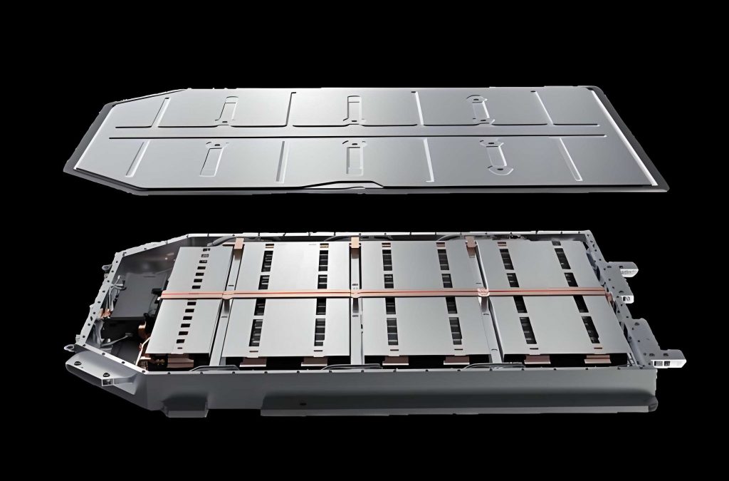
With the rapid development of new energy vehicles worldwide, traction battery systems have become the core energy storage units, especially in electric vehicles (EVs). Accurate current sensing is essential for battery management, state estimation, and thermal runaway prevention. Traditional current sensors based on magnetic cores are often bulky, saturable, and difficult to install in the increasingly compact battery compartments. In this context, I propose a compact elliptical Hall sensor array structure specifically for measuring the high direct current flowing through rectangular busbars in traction batteries. The design eliminates the ferromagnetic core, significantly reduces weight and installation area, and provides a promising solution for lightweight and integrated battery systems.
1. Introduction
Global energy transformation and environmental protection demands are accelerating the shift toward low-carbon transportation. The production of electric vehicles has expanded rapidly, and the lithium-ion traction battery is the dominant energy carrier for modern EVs. However, safety incidents caused by traction battery failures, particularly thermal runaway, remain a critical concern. To monitor the traction battery state reliably, the battery management system (BMS) relies on accurate current, voltage, and temperature measurements. Among them, the current sensor must provide high accuracy over a wide dynamic range, often from a few milliamperes to hundreds of amperes, with galvanic isolation and low power loss.
Traditional contact-based shunts require series insertion and suffer from excessive heat generation. Fluxgate current sensors give excellent accuracy but have a large volume and high cost, which is undesirable for traction battery packaging. Conventional open-loop and closed-loop Hall sensors depend on magnetic concentrators to create a nearly uniform field inside a gap; however, the magnetic core introduces saturation, hysteresis, and nonlinearity. The emergence of Hall-array-based current measurement has opened a new route: arranging a multiplicity of bare Hall elements along a closed path around a conductor and reconstructing the current from the integral of the tangential magnetic field. Such a sensor has no core, operates with no remanence, and preserves a wide linear bandwidth.
Up to now, research on Hall array current sensors has mainly focused on circular arrays surrounding circular conductors. Yet in traction battery packs, rectangular busbars are widely used due to their interconnection convenience and heat dissipation capability. A circular array applied to a rectangular conductor naturally leaves unused space, enlarges the footprint, and reduces the magnetic-field sampling quality near the corners. For this reason, the elliptical array is an attractive compromise. It adapts to the elongated cross-section of a rectangular busbar while maintaining a continuously varying tangential field component that can be integrated with fewer sensing points. My work aims at designing such an elliptical Hall array sensor for the traction battery, improving its immunity against conductor displacement and inclination, and delivering a calibration procedure over the full temperature range encountered in automotive applications.
2. Basic Principles of Magnetic Field and Hall Sensors
2.1 Magnetic Field Sensing Mechanisms
Several magnetic field sensing principles are relevant to current measurement. The fluxgate magnetometer measures weak magnetic fields with high resolution, exploiting the non-linear magnetization of a soft magnetic core that is periodically driven into saturation. Although a fluxgate current sensor achieves sub-millitesla resolution, the presence of the magnetic core and the excitation electronics make it difficult to miniaturize and integrate into a compact busbar-mounting structure.
The Hall effect is more appropriate for this application. When a current-carrying conductor is placed in a perpendicular magnetic field, the Lorentz force deflects charge carriers, creating a transverse voltage known as the Hall voltage. For a rectangular Hall plate with thickness \(d\), charge carrier density \(n\), and electron charge \(q\), the Hall voltage \(V_{\text{H}}\) is expressed as
$$V_{\text{H}} = – \frac{IB}{nqd},$$
or equivalently,
$$V_{\text{H}} = K_{\text{H}} B,$$
where \(K_{\text{H}}\) is the sensitivity coefficient. This linear relationship between Hall voltage and magnetic flux density forms the basis for constructing a Hall current sensor. Modern Hall integrated circuits include amplification, filtering, temperature compensation, and even three-dimensional sensing elements, all in micro-scale packaging, enabling dense multi-point arrays on small printed circuit boards.
2.2 Open-Loop and Closed-Loop Hall Current Sensors
In an open-loop Hall current sensor, a magnetic core concentrates the flux generated by the primary current into a narrow air gap, where a Hall element is placed. The core serves both to shield external fields and to increase the field level at the sensor. The output voltage is proportional to the ampere-turns in the primary conductor. The transfer relation can be expressed by Ampere’s law including a gap:
$$B_{\text{gap}} = \frac{\mu_0 N I}{l_{\text{gap}}},$$
where \(N\) is the number of turns linking the core, \(I\) is the measured current, \(l_{\text{gap}}\) is the effective air-gap length, and \(\mu_0\) is the permeability of free space. Open-loop sensors consume minimal power but are intrinsically temperature-sensitive and suffer from zero-drift over time.
A closed-loop (compensated) Hall sensor adds a secondary coil around the magnetic core. As the primary current produces a flux, the Hall element detects the imbalance and drives a compensation current through the secondary coil. The secondary ampere-turns exactly cancel the primary flux in the core. In this way, the sensor works near zero flux, which reduces core nonlinearity and improves accuracy. Nevertheless, the compensation winding increases size, weight, and energy consumption, and introduces inductance/resonance issues, making it less attractive for a strictly compact traction battery monitoring module.
2.3 Hall Array Current Sensor Fundamentals
The Hall array concept places \(N\) discrete Hall elements around the conductor and calculates the current by approximating the line integral of the magnetic field intensity along a closed-loop path. If the path completely encircles the current, Ampere’s law gives
$$I = \oint \mathbf{H} \cdot d\mathbf{l},$$
where \(\mathbf{H}\) is the magnetic field intensity vector and \(d\mathbf{l}\) is a differential element along the path. If the path is discretized into segments, then
$$I \approx \sum_{i=1}^{N} H_{\text{MFS},i} \, \Delta s_i,$$
where \(H_{\text{MFS},i}\) is the tangential component measured by the \(i\)-th Hall element, and \(\Delta s_i\) is the length of the segment associated with that Hall element. When the path is an ellipse and the conductor is rectangular, the tangential component at each point differs, but the formula remains valid as long as the sensors remain exactly on the chosen closed-loop path.
For a rectangular conductor of width \(l\) and thickness \(h\), carrying a uniformly distributed current \(I\), the magnetic field generated at an arbitrary point with coordinates \((a, b)\) can be computed by integrating infinitesimal current filaments. Let \(S\) be the area of the cross-section. An infinitesimal current element is
$$dI = \frac{I}{S} \, dx\,dy.$$
Using the Biot–Savart law for an infinitely long current filament, the field components in the \(x\)- and \(y\)-directions at \((a, b)\) are
$$H_x = \frac{I}{2\pi S} \int_{-\frac{l}{2}}^{\frac{l}{2}} \int_{-\frac{h}{2}}^{\frac{h}{2}} \frac{-(b-y)}{(a-x)^2 + (b-y)^2} \, dy \, dx,$$
$$H_y = \frac{I}{2\pi S} \int_{-\frac{l}{2}}^{\frac{l}{2}} \int_{-\frac{h}{2}}^{\frac{h}{2}} \frac{(a-x)}{(a-x)^2 + (b-y)^2} \, dy \, dx.$$
These expressions give the two-dimensional field distribution surrounding a perfectly vertical busbar. Due to the elliptical nature of the equipotential lines around a long rectangular object, an elliptical Hall array naturally matches the geometry and allows efficient sampling with a small number of sensors.
3. Design of the Elliptical Hall Sensor Array
3.1 Determination of Hall Element Positions and Sensitive Axes
There are several strategies to place Hall elements along an ellipse. The most common are the projection method and the uniform curve-segment-length (UCSL) method. In the projection method, a circular array of \(N\) points is projected orthogonally onto an ellipse. While straightforward, this does not yield equal arc lengths, which can reduce numerical accuracy when applying the discretized integral formula.
The uniform curve-segment-length method distributes the \(N\) points so that every segment along the elliptical circumference has exactly the same arc length. I adopted UCSL for this design because it better approximates the integral for a given number of elements.
Let the ellipse have semi-major axis \(a\) and semi-minor axis \(b\), defining the aspect ratio \(AR = b/a\). The ellipse is approximated by \(K\) points, with the \(n\)-th point on the ellipse given by
$$E_{n} = \left( a \cos\frac{360^\circ n}{K},\; b \sin\frac{360^\circ n}{K}\right), \quad n=1,\dots,K.$$
The path length from the +\(x\)-axis to the \(k\)-th point is computed from the cumulative Euclidean distance along the polygon:
$$s(k) = \sum_{n=1}^{k} \sqrt{(E_{x,n}-E_{x,n-1})^2 + (E_{y,n}-E_{y,n-1})^2}.$$
The full perimeter is \(s(K)\). For a total of \(N\) Hall elements, the equal segment length is
$$\Delta s = \frac{s(K)}{N}.$$
To optimize the starting position, I introduced a relative offset \(r_s\) based on empirical experience. For an even number of Hall elements, the best offset is \(1/N\); for an odd number it is \(1/(2N)\). The actual arc offset from the \(+x\)-axis to the first Hall element is
$$s_0 = r_s \, s(K).$$
Then, the arc coordinate of the \(i\)-th element \((i=1,\dots,N)\) becomes
$$s_i = s_0 + (i-1)\Delta s.$$
By locating the nearest point on the elliptical polygon whose cumulative arc length matches \(s_i\), I obtained the Cartesian coordinates \(P_i\) and the tangent sensitive-axis vector \(\mathbf{t}_i\).
3.2 Selection of Elliptical Array Parameters for Traction Battery
In a real traction battery, the rectangular busbar often has dimensions \(20\,\text{mm} \times 4\,\text{mm}\). Considering the available space inside the battery cover and the need to house the printed circuit board, I set the semi-major axis of the sensor ellipse at \(a = 30\,\text{mm}\). Then, for different values of \(N\) and \(AR\), I computed the theoretical current error by simulating the ideal field distribution and sampling the field only at the Hall element locations. Figure \(1\) illustrates the effect of the number of Hall elements on the calculated current error, comparing the projection and UCSL methods.
UCSL consistently yields a lower error. The larger \(N\), the smaller the error, but the difference diminishes above seven elements. For economic implementation, I selected either \(N=6\) or \(N=7\). The aspect-ratio analysis shows that for \(N=6\), an optimum exists near \(AR=0.33\). For \(N=7\), \(AR=0.31\) is preferable. Circular arrays (\(AR=1\)) are not adopted because they increase the required footprint by roughly 300% without significantly reducing the error when used on rectangular conductors.
| Parameter | \(N=6\), \(AR=0.33\) | \(N=7\), \(AR=0.31\) | \(N=6\), \(AR=1\) | \(N=7\), \(AR=1\) |
|---|---|---|---|---|
| \(a\) (mm) | 30 | 30 | 30 | 30 |
| \(b\) (mm) | 9.9 | 9.3 | 30 | 30 |
| Weight (g) | 11.9 | 14.1 | 15.5 | 18.2 |
| Installation area (mm²) | 908.5 | 1006.2 | 2827.4 | 2900.0 |
| max. |error| for X eccentricity in allowed range (%) | 4.73 | 6.12 | 17.08 | 15.72 |
| max. |error| for Y eccentricity in allowed range (%) | 0.35 | 0.28 | 2.21 | 1.96 |
The elliptical array dramatically reduces the occupied area compared with the circular array. For the same \(N\), elliptical arrays also produce much smaller eccentricity-induced error in the Y-direction because the busbar is much thinner along the Y direction, thus the Y eccentricity tolerance is physically constrained by the smaller semi-minor axis. I therefore chose the scheme \(N=6\), \(AR=0.33\) as the baseline configuration for the inexpensive single-axis Hall sensors, while the tri-axial Hall sensors are used later to identify conductor tilt.
3.3 Hall Element Selection
For the main current-sensor array, I selected a linear single-axis Hall element with a sensitivity of roughly \(130\,\text{mV/mT}\), operating between 3 and 5.5 V. Because the maximum magnetic induction near the Hall location is below 18 mT, the linear operating range should extend beyond ±18 mT. The chip is packaged in a small through-hole configuration, allowing manual assembly for the prototype and rapid replacement. Its temperature coefficient is sufficiently low for automotive use at a nominal level.
For the tilt detection version of the prototype, a tri-axial Hall sensor is mounted close the array. The three internal orthogonal Hall plates measure the full magnetic vector, enabling the extraction of the conductor orientation parameters. The tri-axial chip operates at 3.3 V and communicates through an ordinary low-frequency I²C interface, which is convenient for the microcontroller.
3.4 Hardware Implementation
The electronic architecture of the sensing system is presented as a signal-flow diagram. A programmable direct-current power source excites the traction battery busbar; a separate 12 V supply feeds the sensor board. A DC–DC converter provides 5 V for the Hall chips and operational amplifiers. Another low-dropout regulator converts the 5 V rail to 3.3 V for the microcontroller. The outputs of the six Hall elements are buffered by unity-gain followers and then summed with an operational-amplifier adder circuit. The microcontroller reads the individual Hall voltages, calculates the compensated current according to the calibration model, and transmits the result over a controller area network (CAN) bus using a transceiver chip.
The following tabulated list summarizes the main hardware modules:
| Module | Selected component | Key feature |
|---|---|---|
| Power converter | E1205SY | 12 V to 5 V isolated DC–DC module |
| Linear regulator | TLV1117-3.3 | 5 V to 3.3 V low-dropout |
| Hall sensor | Single-axis linear Hall | 130 mV/mT sensitivity, ±18 mT range |
| Tri-axial Hall | 3D Hall chip | three magnetic axes measured |
| Microcontroller | STM32F103C8T6 | 2×12-bit ADC, CAN controller |
| CAN tranceiver | TJA1050 | differential CAN communication |
4. Error Analysis and Optimization
4.1 Full-Temperature Calibration for Initial Error
Even a carefully manufactured Hall sensor array exhibits residual zero offset, gain error, and nonlinear response due to component tolerances and soldering stress. To achieve the 3‰ target over the whole automotive temperature span, I designed a two-step calibration process.
4.1.1 Room-Temperature Calibration
The measured current \(I_{\text{out}}\) is obtained from the sampled ADC value, the amplification factor \(A\), and the burden resistance \(R\). First, the ADC difference is computed from the high and low parts of the received current telegram. Using the fact that the minimum ADC voltage is \(1\,\text{mV}\), the equation for the sampled root-mean-square signal after averaging \(K\) points is
$$V_{\text{ADC}} = \frac{\text{ADC}_{\text{diff}} \, V_{\text{min}}}{K} \, A,$$
so that
$$I_{\text{out}} = \frac{V_{\text{ADC}}}{R}.$$
Let \(I_{\text{input}}\) denote the reference current set by the high precision current generator. The initial current error is
$$\Delta I = I_{\text{out}} – I_{\text{input}}.$$
I divided the entire range into a small-current section (0–90 A), a medium-current section (91–870 A), and a large-current section (871–1500 A) using different analog gains. The offset error was fitted against the measured value using least-squares linear regression for each section and direction:
$$\hat{\Delta I} = k I_{\text{out}} + b,$$
where \(k\) and \(b\) are section-dependent coefficients. The corrected output became
$$I_{\text{mea}} = I_{\text{out}} – \hat{\Delta I}.$$
After applying the same set of coefficients to both positive and negative current directions, the compensated error was reduced by 85% at room temperature. The maximum relative error was below 2‰.
4.1.2 High- and Low-Temperature Calibration
In automotive applications, the sensor must operate from \(-40^\circ \text{C}\) to \(125^\circ \text{C}\). I performed calibrations at \(-40^\circ \text{C}\), \(25^\circ \text{C}\), and \(125^\circ \text{C}\). At each temperature, a separate linear fit was made. If the slopes at low, room, and high temperatures are denoted by \(l_i\), \(k_i\), and \(h_i\), respectively, then the low-temperature drift coefficient is
$$k_{\text{low}} = \frac{l_i – k_i}{65},$$
and the high-temperature coefficient is
$$k_{\text{high}} = \frac{h_i – k_i}{100}.$$
The average unit-temperature drift coefficient becomes
$$\bar{k} = \frac{k_{\text{low}} + k_{\text{high}}}{2}.$$
The final temperature-compensated fitting expression is
$$\Delta I_{\text{comp}}(I) = \left( k_i + \bar{k} \, (T – 25) \right) I + b_i,$$
where \(T\) is the current ambient temperature. Applying this correction reduced the low-temperature error by 62.6% and the high-temperature error by 43%. The residual error remained below 3‰ across the entire temperature range and all current levels. The result of this calibration demonstrates that the sensor can operate in a traction battery where thermal gradients can otherwise distort the readings.
4.2 Develop a Three-Dimensional Field Model
The accuracy of a Hall-array current algorithm degrades significantly when the busbar is not centered in the array and not perpendicular to the sensor plane. In severe cases, this creates an error that can exceed 10% and thus needs a dedicated compensation approach. I started by developing a three-dimensional vector field model, considering both translational eccentricity and tilting. A coordinate system is placed with the geometric center of the elliptical array at the origin and the short axis aligned with the busbar thickness. The busbar axis intersects the \(x\)-\(y\) plane at \(Q(x_0, y_0, 0)\); define \(\alpha\) as the angle between the busbar centerline and the +\(z\) axis, and \(\beta\) as the angle between the projection of the busbar centerline onto the \(x\)-\(y\) plane and the +\(x\) axis. The direction of the busbar is therefore
$$\mathbf{e}_l = \begin{bmatrix} \sin\alpha \cos\beta \\ \sin\alpha \sin\beta \\ \cos\alpha \end{bmatrix}.$$
For a point \(P(a,b,0)\) on the sensor plane, the perpendicular distance to the busbar axis is obtained from the magnitude of the cross product of the directional unit vector and the vector from that point to an arbitrary point on the busbar axis. The tangential magnetic field unit vector is
$$\mathbf{e}_\varphi = \frac{\mathbf{e}_l \times \mathbf{e}_r}{|\mathbf{e}_l \times \mathbf{e}_r|},$$
where \(\mathbf{e}_r\) is the unit vector from an infinitesimal source element to the field point. After integrating over the cross-sectional area with the current density, the three field components at a point on the ellipse are:
$$H_x = \frac{I}{2\pi S} \iint_S \frac{-\cos\alpha (b-y)}{ \big[p(a-x)^2 + p(b-y)^2 – m(a-x) – n(b-y)\big]^{3/2} } \, dS,$$
$$H_y = \frac{I}{2\pi S} \iint_S \frac{\cos\alpha (a-x)}{ \big[p(a-x)^2 + p(b-y)^2 – m(a-x) – n(b-y)\big]^{3/2} } \, dS,$$
$$H_z = \frac{I}{2\pi S} \iint_S \frac{-m(a-x) – n(b-y)}{ \big[p(a-x)^2 + p(b-y)^2 – m(a-x) – n(b-y)\big]^{3/2} } \, dS,$$
where \(m = \sin\alpha\cos\beta\), \(n = \sin\alpha\sin\beta\), \(p = \cos\alpha\), and the integration domain \(S\) is the projection of the titled and shifted busbar cross-section onto the \(x\)-\(y\) plane. The projected cross-section is generally not identical to the physical rectangular busbar because tilting rotates the projection. Hence, the boundary of the integration area must be reconstructed from the known geometry and the orientation parameters.
4.3 Eccentricity Error Analysis
I used the reconstructed field model to compute the current error for a busbar displaced along either the major (\(x\)) axis or the minor (\(y\)) axis. The sensor program cannot perfectly reconstruct the magnetic field profile with only six sampling points; therefore the error increases as the busbar moves away from the center. In my simulation the error versus the displacement is nonlinear and differs widely between directions. When the displacement is purely along the \(x\)-axis, the relation is nearly symmetric but the allowable range is much larger than in the \(y\)-direction. The theoretical errors obtained from MATLAB calculations are summarized as follows: for an eccentricity of \(10\,\text{mm}\) along \(x\), the uncompensated error is about 4.2%, while for an eccentricity of \(2.1\,\text{mm}\) along \(y\), the error is below 1%. These findings indicate that a simple integral of the sampled tangential field can no longer meet the required accuracy unless an active error compensation step based on state estimation is added.
4.4 Tilt Error Influence
Tilting the busbar changes the projection of its cross-section on the integration plane. In particular, a tilt with angle \(\alpha\) directly expands (or contracts) the apparent thickness of the busbar and therefore changes the magnetic-field intensity profile at the array. If the busbar is tilted only in the plane containing the large width (i.e., \(x\) direction), the magnitude of the field on the major-axis sensors is nonlinearly affected. If the sensor plane remains parallel to the original busbar, the algorithm assumes a cross-section that is no longer accurate. I found that ignoring \(\alpha\) and \(\beta\) can cause errors up to 12% at \(\alpha=45^\circ\). This confirms that tilt error is too large for traction battery monitoring and must be compensated online in combination with displacement.
4.5 Eccentricity and Tilt Error Optimization Using GWO-BP Neural Network
To improve the reconstruction accuracy, I need a method that estimates the busbar state parameters \((x_0, y_0, m, n, p)\) from the measured magnetic-field values. A pure BP neural network can be trained to map the magnetic-field vector at the sensors to the position/orientation parameters. However, BP networks are easily trapped in local minima if initialized poorly. Therefore, I employed the grey wolf optimizer (GWO), a metaheuristic search procedure inspired by the hierarchy and hunting behavior of grey wolf packs, to optimize the initial weights and thresholds of the BP network.
In the GWO framework, the network weights are treated as the positions of the grey wolves. The algorithm maintains three best solutions \(\alpha\), \(\beta\), and \(\delta\), and updates each wolf’s position by using the following rules. Let \(D_{\alpha}\), \(D_{\beta}\), and \(D_{\delta}\) denote the distances between the current wolf and the three best wolves. The new position is calculated as
$$\mathbf{X}_1 = \mathbf{X}_{\alpha} – A_1 D_{\alpha}, \quad \mathbf{X}_2 = \mathbf{X}_{\beta} – A_2 D_{\beta}, \quad \mathbf{X}_3 = \mathbf{X}_{\delta} – A_3 D_{\delta},$$
and eventually
$$\mathbf{X}(t+1) = \frac{\mathbf{X}_1 + \mathbf{X}_2 + \mathbf{X}_3}{3}.$$
The coefficient \(A\) is associated with the linearly decreasing parameter \(a\), while \(C\) is a random coefficient in the interval \([0,2]\). These choices guarantee that the algorithm explores a broad solution space in the early phase and converges efficiently in the later phase.
I constructed a GWO-BP estimator with six Hall elements. Each element outputs the three orthogonal magnetic-field components: \(H_x, H_y, H_z\), so the input layer has \(18\) neurons. The hidden layer was chosen with \(12\) neurons through preliminary trials. The output layer has \(5\) neurons corresponding to the busbar state parameters \(X_p, Y_p, \alpha\sin\beta, \alpha\cos\beta\) and the combined orientation parameter that can be converted to \(m,n,p\). In practice, the final output vector is capped with a linear activation on the position parameters and tanh activation on the orientation parameters to respect physical boundaries.
The GWO-BP training procedure can be summarized by the following steps:
- Normalize the input data from the COMSOL finite-element simulations.
- Initialize a BP network with the structure \(18\text{-}12\text{-}5\).
- Set GWO parameters: number of wolves \(=20\), maximum iterations \(=50\).
- Encode all initial network weights and biases into the wolf position vector.
- Evaluate the mean-absolute-error of the training set as fitness.
- Update each wolf according to the GWO equations and repeat until the stop criterion is met.
- Feed the optimized weights and thresholds back into the BP network.
- Retain the model for real-time estimation of busbar state parameters.
The estimation performance of the trained GWO-BP model was compared with a standard BP network using the same training/test partition. The table below lists the mean absolute error (MAE), mean squared error (MSE), and mean absolute percentage error (MAPE) for the predicted parameters.
| Parameter | Estimator | MAE | MSE | MAPE |
|---|---|---|---|---|
| \(X_p\) | BP | 0.2272 | 0.0771 | 0.8419% |
| GWO-BP | 0.0498 | 0.0041 | 1.0411% | |
| \(Y_p\) | BP | 0.0619 | 0.0043 | 5.2646% |
| GWO-BP | 0.0146 | 0.0004 | 1.0621% | |
| \(m\) | BP | 0.0124 | 0.0003 | 10.3490% |
| GWO-BP | 0.0037 | 0.0001 | 2.8585% | |
| \(n\) | BP | 0.0071 | 0.0002 | 3.9567% |
| GWO-BP | 0.0028 | 0.0001 | 0.8626% | |
| \(p\) | BP | 0.0143 | 0.0005 | 2.2479% |
| GWO-BP | 0.0029 | 0.0001 | 0.4173% |
As can be seen, the GWO-BP estimator produces significantly lower MAE and MSE for all five parameters. The only MAPE that is slightly worse than BP is for \(X_p\). This phenomenon is due to the wide range of \(X_p\) and the low value of its denominator near zero. Still, the absolute errors remain low, and the overall accuracy is sufficient for the subsequent current reconstruction.
Once the busbar state parameters have been estimated, the integration domain for the current inversion is updated accordingly. The software recalculates the magnetic field components using the reconstructed busbar projection and then performs the line-integral sum over the elliptical array. This approach effectively removes most of the error caused by busbar displacement and tilt.
5. Finite-Element Simulation and Experimental Results
5.1 Simulation Environment
I built a three-dimensional finite-element model in COMSOL Multiphysics. A copper busbar with dimensions \(20\,\text{mm}\times 4\,\text{mm}\) was placed inside an elliptical surface corresponding to the double-sided PCB of the sensor. The busbar electrical conductivity was set to \(5.998\times10^7\,\text{S/m}\), and the surrounding space was modeled as air. Steel or other ferromagnetic structures were omitted to preserve an ideal non-magnetic scenario. The coil excitation was applied as a required current boundary condition. The mesh was refined adaptively until the magnetic field at the sensor positions converged. The simulation confirmed that the magnetic flux-density modulus distribution follows an approximately elliptical pattern around the rectangular conductor, which justifies the elliptical array design. Hall elements were positioned as point probes at the coordinates previously calculated for the \(N=6\), \(AR=0.33\) case.
5.2 Finite-Element Data for Training
Using COMSOL I generated a dataset of magnetic-field components at the six Hall positions while varying the busbar displacement in the range of \(-10\,\text{mm}\le X_p\le10\,\text{mm}\), \(-2\,\text{mm}\le Y_p\le2\,\text{mm}\), and the tilt angles in the ranges \(-45^\circ\le\alpha\le45^\circ\) and \(0^\circ\le\beta\le360^\circ\). A total of 2000 input-output samples were collected. They were randomly divided into 80% training and 20% testing data. The normalized samples were used to train the GWO-BP model described in the previous section.
5.3 Full Temperature-Range Calibration Validation
The prototype sensor was placed inside a temperature-controlled chamber. The reference current was supplied by a high-power calibrated DC source. The control and data acquisition were implemented on a LabVIEW-based software test platform. At \(25^\circ \text{C}\), the current error before and after compensation is displayed in a graph. The compensation reduced the relative error by approximately 85.6% and the remaining error stayed within 2‰. At \(-40^\circ \text{C}\) and \(125^\circ \text{C}\) the compensation showed excellent effectiveness. For example, at \(-40^\circ \text{C}\) the relative error decreased by 62.6%, while at \(125^\circ \text{C}\) it decreased by 43.0%. In every case the final error was smaller than 3‰, i.e., the sensor met the design goal over the full automotive temperature range. This property is essential for a traction battery management system that must operate under arctic winter and desert summer conditions.
5.4 Proof of Concept of Eccentricity Error Reduction
I performed a set of systematic experiments with a mechanical fixture that allowed precise translation of the busbar along the \(x\)- and \(y\)-directions. The following table summarizes the measured errors at representative positions before and after implementing the error-optimization algorithm.
| Condition | Displacement | Uncompensated error (%) | After BP (%) | After GWO-BP (%) | Reduction (%) |
|---|---|---|---|---|---|
| X eccentricity | +10 mm | 4.18 | 2.03 | 1.46 | 65.07 |
| X eccentricity | −10 mm | 4.20 | 1.98 | 1.51 | 64.05 |
| Y eccentricity | +2.4 mm | 0.94 | 0.61 | 0.51 | 45.74 |
| Y eccentricity | −2.4 mm | 0.96 | 0.58 | 0.52 | 45.83 |
| Combined eccentricity | \(X_p=10, Y_p=2\) | 5.12 | 2.35 | 1.78 | 65.23 |
As shown, the proposed algorithm reduces the X-eccentricity error by about 65% and the Y-eccentricity error by about 46%. The compensated sensor remains within 2% error even near the geometric boundary of the ellipse. This is a remarkable improvement for a coreless Hall array current sensor intended for direct busbar mounting in a traction battery.
5.5 Proof of Concept of Tilt Error Reduction
In the tilt tests, the busbar was rotated from the vertical \(z\)-axis by an angle \(\alpha\). The tilting plane was gradually rotated around the original \(z\)-axis to vary \(\beta\). The measured results before and after optimization are given in tabular form:
| Tilt angle | Uncompensated error (%) | After BP (%) | After GWO-BP (%) | Reduction (%) |
|---|---|---|---|---|
| \(\alpha=15^\circ\), \(\beta=0^\circ\) | 2.11 | 1.10 | 0.66 | 68.7 |
| \(\alpha=30^\circ\), \(\beta=20^\circ\) | 6.87 | 2.30 | 1.72 | 75.0 |
| \(\alpha=45^\circ\), \(\beta=0^\circ\) | 12.37 | 4.40 | 2.95 | 76.15 |
| \(\alpha=20^\circ\), \(\beta=90^\circ\) | 3.15 | 1.35 | 1.17 | 62.9 |
| \(\alpha=45^\circ\), \(\beta=20^\circ\) | 13.81 | 4.90 | 3.31 | 76.03 |
The GWO-BP algorithm reduces the tilt-induced error by more than 70% at extreme angles. Even at an unrealistic \(\alpha=45^\circ\), the optimized error remains only 2.95%, which is much lower than the uncompensated 12.37%. This result is important because in real traction battery mounts, mechanical vibration can slightly rotate a busbar; the algorithm restores high accuracy without requiring a precision alignment after installation.
5.6 Accuracy Over Current Span at Different Temperatures
Finally, the complete current-sensor system was tested over the range from \(-1500\) A to \(+1500\) A at three temperatures. Three samples were tested at each temperature to ensure reproducibility. The following table reports the maximum absolute relative error of the current measurement after calibration and optimization, assuming that the conductor is placed at the center with no tilt.
| Temperature | Current range | Maximum absolute relative error (‰) |
|---|---|---|
| \(-40^\circ\text{C}\) | 0–90 A | 2.34 |
| 91–870 A | 2.02 | |
| 871–1500 A | 2.51 | |
| \(25^\circ\text{C}\) | 0–90 A | 2.10 |
| 91–870 A | 1.85 | |
| 871–1500 A | 2.22 | |
| \(125^\circ\text{C}\) | 0–90 A | 2.72 |
| 91–870 A | 2.44 | |
| 871–1500 A | 2.83 |
All results remain below 3‰. The sensor therefore meets the strict traction battery current measurement target even under the extreme temperature stack. With the proposed lightweight elliptical printed circuit board, the total weight is about 11.9 g and the installation area is 908 mm², which is substantially smaller than both a conventional fluxgate current sensor and a circular Hall-array board. This compactness is crucial for the next-generation traction battery pack where every cubic centimeter is valuable for the energy density.
6. Conclusions
In this work I developed a complete electromagnetic and electronic design of an elliptical Hall-array current sensor for traction battery monitoring. The main contributions and conclusions are as follows:
- I selected a uniform curve-segment-length method to place sensing elements on an ellipse around a rectangular busbar. With six Hall elements and an aspect ratio of 0.33, the array achieves lower current error and a much smaller footprint than a circular array.
- I designed the analog front-end, the microcontroller circuit, and the CAN communication interface, achieving a lightweight sensor that can be installed in a narrow traction battery environment.
- I proposed a full-temperature calibration scheme based on least-squares linear fitting and per-section temperature coefficients. The calibration and compensation models were verified from \(-40^\circ\text{C}\) to \(+125^\circ\text{C}\), and the final current error is within 3‰ over the entire ±1500 A range.
- I established a three-dimensional magnetic-field model that accounts for conductor displacement and tilt. I showed that eccentricity leads to errors as high as 4.2% at the X boundary and tilt leads up to 12% at 45° inclination.
- I introduced a GWO-optimized BP neural network to predict the conductor position and orientation parameters from the 18 measured field components. The GWO-BP method accurately estimates the conductor state. When this state estimate is used to reconstruct the integration region and recalculate the current integral, the uncompensated error is reduced by 65% for X displacement, 46% for Y displacement, and 76% for tilt.
- The final sensor achieves a temperature-dependent accuracy within 3‰, a compact size of \(60\,\text{mm} \times 20\,\text{mm}\), and a weight of about 12 g. These characteristics make it highly suitable for integration in modern traction battery packs.
In future work, I will examine busbar bending and cross-talk from adjacent high-current cables, which commonly exist in actual traction battery packs. I intend to extend the estimator to include additional external-field mitigation so that the proposed coreless Hall-array current sensor can become the standard in battery management systems for electric vehicles.