
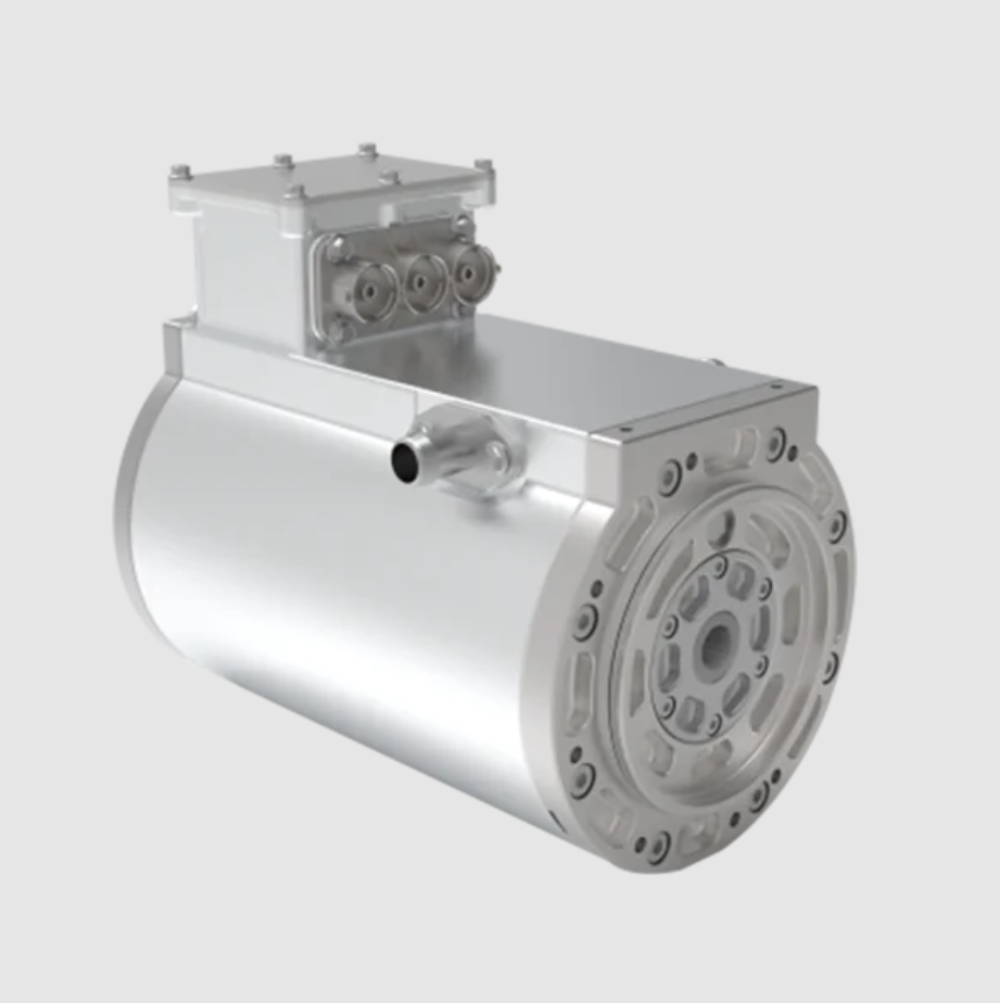
In this work, I focus on the thermal state estimation of a permanent magnet synchronous motor, especially the rotor temperature distribution. Excessive temperature in a permanent magnet synchronous motor can cause irreversible demagnetization of the permanent magnets. For safety-critical applications such as electric vehicles and aircraft drives, the permanent magnet synchronous motor must remain within a safe operating temperature range. Because the magnets are mounted on the rotor, direct measurement of magnet temperature is difficult due to rotation. Thermal-resistance-network-based observers are computationally expensive, and some thermal resistance parameters are hard to obtain. To address this problem, I use the no-load back electromotive force method to estimate the average rotor temperature of the permanent magnet synchronous motor. On this basis, I monitor the housing temperature comprehensively and estimate the axial rotor temperature from the axial temperature distribution relationship between the housing and the rotor. This method solves the problem that the axial rotor temperature is difficult to measure directly. I validate the proposed method on a motor test platform.
The permanent magnet synchronous motor has the advantages of high power density, high efficiency, and fast dynamic response, and it is widely used in electric vehicles, industrial drives, and wind power generation. During operation, power losses increase the temperature of the rotor permanent magnets. If the magnet temperature becomes too high, demagnetization occurs, which directly affects the safe operation and service life of the permanent magnet synchronous motor. Therefore, the permanent magnet synchronous motor must be designed so that the permanent magnets operate within a safe temperature region. Common detection methods for permanent magnet synchronous motor temperature can be divided into contact and non-contact types.
Thermocouples are often used for stator temperature detection, but because there is an air gap between the stator and the rotor, the temperatures are different. Contact-type rotor temperature measurement often requires slip rings to transmit temperature signals, but slip rings have a short lifetime and are difficult to use in long-life applications. To solve this problem, wireless transmission methods have been proposed, which do not require mechanical transmission devices and therefore avoid the lifetime problem. However, the internal space of the permanent magnet synchronous motor is narrow, and installing temperature measurement and signal transmission modules requires modification or customization of the motor. The implementation difficulty and cost are high, and maintenance and fault repair are complex.
To avoid modifying the permanent magnet synchronous motor, non-contact temperature measurement methods have been proposed, such as thermal circuit methods, no-load back electromotive force methods, and finite element simulation methods. The thermal circuit method establishes a thermal circuit model based on the motor structure and material properties of each part, and uses mathematical calculation or simulation to predict the temperature at each position of the motor. This method can obtain detailed axial and radial temperatures of the permanent magnet synchronous motor, which is beneficial for power density optimization. However, the thermal circuit method is based on a detailed understanding of the motor structure and material properties, and this information may not be fully available in practical applications. At the same time, because the permanent magnet synchronous motor in electric vehicles and aircraft often has a large number of pole pairs, the thermal circuit model calculation is very complex. Finite element simulation can obtain the temperature at each position of the permanent magnet synchronous motor, but the computational burden is very large, and the simulation environment differs greatly from the actual working condition, which may cause large errors between the estimated temperature and the actual temperature.
To solve the problems of information acquisition and computation, a no-load back electromotive force method has been proposed to estimate the rotor temperature of a permanent magnet synchronous motor. This method uses the approximate inverse relationship between the permanent magnet flux linkage and temperature. By measuring the back electromotive force, the flux linkage at the current temperature is calculated and compared with the flux linkage at room temperature to obtain the current temperature. This method does not require complex calculation, and the signal acquisition is relatively simple. It has certain advantages for rotor temperature estimation of the permanent magnet synchronous motor. However, this method requires the no-load back electromotive force of the motor, and its test must be carried out under specific conditions. Moreover, the temperature measured by this method is the average temperature of the rotor.
To minimize the impact on the permanent magnet synchronous motor and simultaneously estimate the rotor temperature distribution, I investigate a back electromotive force method based on measuring the housing temperature distribution to estimate the axial rotor temperature distribution. First, I obtain the average temperature of the permanent magnets from the back electromotive force of the permanent magnet synchronous motor. Then, by analyzing the thermal resistance model of the motor and applying the law of conservation of heat flow, I obtain the axial temperature distribution law. Thus, by detecting the surface temperature of the motor, I can estimate the axial temperature distribution of the rotor. Finally, I experimentally verify the method.
Back Electromotive Force Principle for Rotor Temperature Estimation
In a permanent magnet synchronous motor, the permanent magnets exhibit reversible demagnetization as the operating temperature increases. The residual magnetic flux density decreases with increasing temperature. The relationship can be expressed as
$$B_r(t_2) = B_r(t_1)\left\{1 + \alpha\left[T(t_2) – T(t_1)\right]\right\}$$
where \(\alpha\) is the temperature coefficient of the permanent magnet, which can be obtained from the motor manufacturer. In my experimental permanent magnet synchronous motor, \(\alpha = 0.115\%\). \(T(t_1)\) and \(T(t_2)\) are the permanent magnet temperatures at times \(t_1\) and \(t_2\), respectively. \(B_r(t_1)\) and \(B_r(t_2)\) are the residual magnetic flux densities at times \(t_1\) and \(t_2\), respectively. Equation (1) can be rewritten as
$$T(t_2) = \frac{1}{\alpha}\left[\frac{B_r(t_2)}{B_r(t_1)} – 1\right] + T(t_1)$$
The no-load back electromotive force of the permanent magnet synchronous motor can be expressed as
$$E_\phi = 4.44 N k_{y1} k_{q1} \frac{n}{60 P} K \Phi \frac{b_{m0} B_r A_m}{\sigma_0}$$
where \(n\) is the motor speed. Once the permanent magnet synchronous motor design is completed, all parameters in the above equation except \(B_r\) and \(n\) no longer change. Therefore, the ratio of the residual magnetic flux density at \(t_1\) and \(t_2\) can be expressed as
$$\frac{B_r(t_2)}{B_r(t_1)} = \frac{E_\phi(t_2)}{E_\phi(t_1)} \cdot \frac{\omega(t_1)}{\omega(t_2)}$$
Substituting equation (4) into equation (2), the rotor temperature of the permanent magnet synchronous motor at time \(t_2\) is
$$T(t_2) = \frac{1}{\alpha}\left[\frac{E_\phi(t_2)\omega(t_1)}{E_\phi(t_1)\omega(t_2)} – 1\right] + T(t_1)$$
Therefore, as long as the no-load back electromotive force at times \(t_1\) and \(t_2\) is measured, the motor temperature at time \(t_2\) can be obtained. This is the core principle I use for the permanent magnet synchronous motor rotor temperature estimation.
| Symbol | Meaning | Unit |
|---|---|---|
| \(B_r\) | Residual magnetic flux density of permanent magnet | T |
| \(\alpha\) | Temperature coefficient of permanent magnet | 1/°C |
| \(T\) | Temperature | °C |
| \(E_\phi\) | No-load back electromotive force | V |
| \(\omega\) | Angular speed | rad/s |
| \(n\) | Rotational speed | r/min |
| \(N\) | Number of series turns per phase | — |
| \(k_{y1}\) | Fundamental winding factor for pitch | — |
| \(k_{q1}\) | Fundamental winding factor for distribution | — |
| \(P\) | Number of pole pairs | — |
| \(K\) | Thermal conductivity | W/(m·K) |
| \(R\) | Thermal resistance | K/W |
| \(G\) | Thermal conductance | W/K |
| \(\Phi\) | Heat flow | W |
Testing Platform and Back Electromotive Force Measurement
Conventional drag-type motor back electromotive force measurement requires a dragging device to rotate the motor under test to a set speed and then detect the no-load output voltage of the motor under test. This method cannot realize loaded operation of the permanent magnet synchronous motor. To make it convenient to detect the back electromotive force of the permanent magnet synchronous motor under load conditions, I designed a motor test platform. The motor under test is fixed to a virtual load through a coupling. During normal operation, the virtual load controller is in current control mode and provides a load to the motor under test. When the virtual load controller switches to speed control mode, the virtual load motor becomes a dragging device for measuring the back electromotive force. Thus, the permanent magnet synchronous motor can be tested conveniently.
The initial back electromotive force \(E_\phi(t_1)\) and the back electromotive force \(E_\phi(t_2)\) after loaded operation until time \(t_2\) are measured according to the following procedure. First, the motor under test is dragged by the virtual load to a fixed speed, and the terminal voltage is recorded as \(E_\phi(t_1)\). Then the virtual load is switched back to current control mode, and the permanent magnet synchronous motor operates under the desired load. After a specified time \(t_2\), the virtual load is switched to speed control mode again, and the back electromotive force \(E_\phi(t_2)\) is measured at the same speed. Finally, using equation (5), the average rotor temperature at time \(t_2\) is calculated.
| Parameter | Value | Unit |
|---|---|---|
| Rated power | 7.5 | kW |
| Rated speed | 2000 | r/min |
| Number of pole pairs | 4 | — |
| Cooling condition | Natural cooling | — |
| Ambient temperature | 23 | °C |
| Permanent magnet temperature coefficient | 0.115 | %/°C |
Thermal Resistance Analysis of the Permanent Magnet Synchronous Motor
To obtain the temperature distribution relationship between the housing and the rotor, I establish a thermal resistance model of the permanent magnet synchronous motor. The experimental motor is a 4-pole-pair permanent magnet synchronous motor. The radial thermal circuit model includes the housing, stator, air gap, rotor, and permanent magnets. The thermal resistance of the housing and stator can be calculated by
$$R = \frac{1}{2\pi K L}\ln\frac{r_{\mathrm{out}}}{r_{\mathrm{in}}}$$
where \(K\) is the thermal conductivity, \(L\) is the axial length of the part, and \(r_{\mathrm{out}}\) and \(r_{\mathrm{in}}\) are the outer and inner radii of the hollow cylinder, respectively. The rotor structure has double-layer magnets. Following the modeling method for the permanent magnet synchronous motor, the radial thermal resistance model of the rotor is obtained. The thermal resistance of each region can be uniformly calculated by
$$R_i = \frac{\ln(r_{\mathrm{out}}/r_{\mathrm{in}})}{2\pi K L}\cdot \frac{2\pi}{2 n_p \theta}$$
where \(\theta\) is the angle occupied by the region and \(n_p\) is the number of pole pairs. In my experimental permanent magnet synchronous motor, \(n_p = 4\). The parameters of each region are listed in the following table. According to the series-parallel analysis method of thermal resistance, the total radial thermal resistance of the rotor can be simplified as
$$R_{r7} = R_{10} + \frac{1}{\frac{2}{R_9} + \frac{2}{R_8} + \frac{1}{R_7 + R_6} + \frac{1}{\frac{2}{R_2} + \frac{1}{R_1 + R_3 + R_4 + R_5}}}$$
| Region | Inner radius | Outer radius | Thermal conductivity | Angle |
|---|---|---|---|---|
| \(R_1\) | \(r_1\) | \(r_2\) | \(K_{\mathrm{Fe}}\) | \(\theta_1 + 2\theta_2 + 2\theta_3\) |
| \(R_2\) | \(r_1\) | \(r_5\) | \(K_{\mathrm{Fe}}\) | \(2\theta_4 + 2\theta_5\) |
| \(R_3\) | \(r_2\) | \(r_3\) | \(K_{\mathrm{Fe}}\) | \(2\theta_3\) |
| \(R_4\) | \(r_3\) | \(r_4\) | \(K_{\mathrm{Fe}}\) | \(\theta_1 + 2\theta_2 + 2\theta_3\) |
| \(R_5\) | \(r_4\) | \(r_5\) | \(K_{\mathrm{PM}}\) | \(\theta_1 + 2\theta_2 + 2\theta_3\) |
| \(R_6\) | \(r_5\) | \(r_6\) | \(K_{\mathrm{Fe}}\) | \(\theta_1\) |
| \(R_7\) | \(r_6\) | \(r_7\) | \(K_{\mathrm{PM}}\) | \(2\theta_2 + 2\theta_3\) |
| \(R_8\) | \(r_5\) | \(r_7\) | \(K_{\mathrm{Fe}}\) | \(2\theta_4 + 2\theta_5\) |
| \(R_9\) | \(r_5\) | \(r_7\) | \(K_{\mathrm{Fe}}\) | \(\theta_1 + 2\theta_2 + 2\theta_3 + 2\theta_4 + 2\theta_5\) |
| \(R_{10}\) | \(r_7\) | \(r_8\) | \(K_{\mathrm{Fe}}\) | \(\theta_1 + 2\theta_2 + 2\theta_3 + 2\theta_4 + 2\theta_5\) |
The axial thermal resistance model of the experimental permanent magnet synchronous motor can be calculated by the conduction thermal resistance formula for a flat plate. To study the axial temperature gradient of the motor, I divide the motor into four nodes in the axial direction, and the thermal resistance between every two nodes is evenly distributed. Therefore, the axial thermal resistance in the same part is the same. Combining the radial thermal resistance and the axial thermal resistance of the permanent magnet synchronous motor, and simplifying the series-parallel relationships into one thermal resistance for convenience, I obtain the equivalent thermal resistance model of the motor. The losses of each part are obtained by electromagnetic simulation in finite element software and are evenly distributed among the axial nodes. According to the node temperature equation
$$G_{12\times 12}T_{12\times 1} = \Phi_{12\times 1}$$
where \(G_{12\times 12}\) is the thermal conductance matrix and \(\Phi_{12\times 1}\) is the heat flowing into the nodes plus the heat generated by the nodes themselves. The thermal conductance matrix is structured as a banded matrix reflecting the axial and radial connections among the four axial sections of the permanent magnet synchronous motor. The heat flow vector includes the losses of the stator, rotor, and permanent magnets, as well as the boundary heat exchange with the ambient air and the housing. Solving this linear system gives the temperature at each node.
$$G_{12\times 12}=
\begin{bmatrix}
G_{\mathrm{nei}} & -G_1 & 0 & 0 & -G_5 & 0 & 0 & 0 & 0 & 0 & 0 & 0\\
-G_1 & G_{\mathrm{nei}} & -G_1 & 0 & 0 & -G_5 & 0 & 0 & 0 & 0 & 0 & 0\\
0 & -G_1 & G_{\mathrm{nei}} & -G_1 & 0 & 0 & -G_5 & 0 & 0 & 0 & 0 & 0\\
0 & 0 & -G_1 & G_{\mathrm{nei}} & 0 & 0 & 0 & -G_5 & 0 & 0 & 0 & 0\\
-G_5 & 0 & 0 & 0 & G_{\mathrm{nei}} & -G_2 & 0 & 0 & -G_6 & 0 & 0 & 0\\
0 & -G_5 & 0 & 0 & -G_2 & G_{\mathrm{nei}} & -G_2 & 0 & 0 & -G_6 & 0 & 0\\
0 & 0 & -G_5 & 0 & 0 & -G_2 & G_{\mathrm{nei}} & -G_2 & 0 & 0 & -G_6 & 0\\
0 & 0 & 0 & -G_5 & 0 & 0 & -G_2 & G_{\mathrm{nei}} & 0 & 0 & 0 & -G_6\\
0 & 0 & 0 & 0 & -G_6 & 0 & 0 & 0 & G_{\mathrm{nei}} & -G_3 & 0 & 0\\
0 & 0 & 0 & 0 & 0 & -G_6 & 0 & 0 & -G_3 & G_{\mathrm{nei}} & -G_3 & 0\\
0 & 0 & 0 & 0 & 0 & 0 & -G_6 & 0 & 0 & -G_3 & G_{\mathrm{nei}} & -G_3\\
0 & 0 & 0 & 0 & 0 & 0 & 0 & -G_6 & 0 & 0 & -G_3 & G_{\mathrm{nei}}
\end{bmatrix}$$
$$\Phi_{12\times 1}=
\begin{bmatrix}
T_fG_7 + T_{\mathrm{air}}G_4 + \Phi_1\\
T_{\mathrm{air}}G_4 + \Phi_1\\
T_{\mathrm{air}}G_4 + \Phi_1\\
T_bG_8 + T_{\mathrm{air}}G_4 + \Phi_1\\
T_fG_7 + \Phi_2\\
\Phi_2\\
\Phi_2\\
T_bG_8 + \Phi_2\\
T_fG_7 + \Phi_3\\
\Phi_3\\
\Phi_3\\
T_bG_8 + \Phi_3
\end{bmatrix}$$
For the permanent magnet synchronous motor, the axial temperature relationship between the housing surface and the rotor is calculated from the equivalent thermal resistance model. The temperatures at the four axial sections \(T_1\) to \(T_4\) show that the rotor and the housing have different temperatures at the same axial section. As the axial position changes, the temperature changes. The temperature is higher in the middle of the motor and lower at both ends, and the temperatures at the two ends are not equal. However, the rotor temperature variation with axial position is basically consistent with that of the housing. Therefore, the rotor temperature variation law can be obtained from the housing axial temperature variation law. This is the key idea of my estimation method.
Because the back electromotive force method can only obtain the average rotor temperature, and the average of the node temperatures along the rotor axis is the average rotor temperature, I analyze the axial temperature distribution of the rotor and the housing together with their respective average values. The differences between the temperatures of the four axial nodes and the average temperature are listed in the table below.
| Position | Housing temperature deviation (°C) | Rotor temperature deviation (°C) |
|---|---|---|
| \(T_1\) | −2.208 | −4.073 |
| \(T_2\) | 0.1825 | 0.5575 |
| \(T_3\) | 1.1525 | 2.2375 |
| \(T_4\) | 0.8725 | 1.2775 |
I perform a linear fit on the data in the table and obtain
$$\Delta T_{\mathrm{rotor}} = 1.8275 \Delta T_{\mathrm{stator}}$$
where \(\Delta T\) is the difference between each node temperature and the average temperature. The coefficient of determination \(R^2\) of the fit reaches 0.9928, which indicates a good fit. After obtaining the fitting equation, I can apply the detected axial housing temperature to the estimation of the axial rotor temperature. First, I average the detected housing temperature data to obtain the difference between each node and the average housing temperature. Then, according to equation (11), I obtain the difference between each rotor node and the average rotor temperature. Finally, I obtain the average rotor temperature by the back electromotive force method. In this way, I obtain the estimated temperature of each node in the rotor. This procedure is summarized in the following steps.
| Step | Operation | Output |
|---|---|---|
| 1 | Measure no-load back electromotive force at initial temperature | \(E_\phi(t_1)\), \(T(t_1)\) |
| 2 | Operate the permanent magnet synchronous motor under load | Loaded thermal state |
| 3 | Measure no-load back electromotive force again | \(E_\phi(t_2)\) |
| 4 | Calculate average rotor temperature | \(T(t_2)\) from equation (5) |
| 5 | Measure housing temperatures at four axial positions | \(T_{\mathrm{hs},1}\) to \(T_{\mathrm{hs},4}\) |
| 6 | Calculate housing temperature deviations | \(\Delta T_{\mathrm{stator},i}\) |
| 7 | Apply fitting equation | \(\Delta T_{\mathrm{rotor},i} = 1.8275 \Delta T_{\mathrm{stator},i}\) |
| 8 | Add average rotor temperature | \(T_{\mathrm{rotor},i} = T(t_2) + \Delta T_{\mathrm{rotor},i}\) |
Experimental Validation of the Permanent Magnet Synchronous Motor Rotor Temperature Estimation
To complete the motor temperature test experiment, I built a back-to-back motor test platform. The housing of the experimental permanent magnet synchronous motor is provided with four temperature measurement planes at equal distances in the axial direction. On each measurement plane, one thermocouple is installed on the front side and one on the top side to detect the radial temperature distribution. The operating conditions of the permanent magnet synchronous motor are listed in the following table.
| Parameter | Value | Unit |
|---|---|---|
| Speed | 2000 | r/min |
| Cooling condition | Natural cooling | — |
| Power | 7.5 | kW |
| Ambient temperature | 23 | °C |
The back electromotive force of the experimental permanent magnet synchronous motor is measured at room temperature (0 min), after 60 min of operation, and at thermal equilibrium (90 min). The measured values are used to calculate the average rotor temperature at 60 min and at thermal equilibrium. Using equation (5), I obtain
$$T_{60\,\mathrm{min}} = \frac{1}{-0.115\%}\left(\frac{132.14}{139.28} – 1\right) + 23 = 67.58\,^\circ\mathrm{C}$$
$$T_{\mathrm{equilibrium}} = \frac{1}{-0.115\%}\left(\frac{130.11}{139.28} – 1\right) + 23 = 80.25\,^\circ\mathrm{C}$$
Based on the fitting curve, I estimate the axial temperature distribution of the rotor of the experimental permanent magnet synchronous motor. The rotor temperature distribution shows the same trend as the housing temperature distribution and follows the relationship in equation (11). This confirms that the axial rotor temperature can be reconstructed from the housing temperature measurements.
To verify the feasibility of the proposed rotor axial temperature estimation method, I modified the rotor of the experimental permanent magnet synchronous motor. Three temperature sensors were installed in the end shielding plates at each end of the rotor to directly measure the rotor temperature. The output signals pass through wiring holes and a hollow shaft to a conditioning board in a protective box. The signals are sent to a host computer on the stator side via Bluetooth. This direct measurement provides an independent reference for the estimated rotor temperatures.
The estimated and measured rotor temperatures at two time instants are compared. At 60 min, the errors between the estimated and measured values at the front and rear ends of the rotor are 0.65 °C and 1.87 °C, respectively. At thermal equilibrium, the corresponding errors are 1.2 °C and 1.1 °C. Therefore, the rotor temperature estimation method proposed in this work has a small error before and after thermal equilibrium. The following table summarizes the comparison.
| Time | Rotor end | Estimated temperature (°C) | Measured temperature (°C) | Error (°C) |
|---|---|---|---|---|
| 60 min | Front | — | — | 0.65 |
| 60 min | Rear | — | — | 1.87 |
| Thermal equilibrium | Front | — | — | 1.2 |
| Thermal equilibrium | Rear | — | — | 1.1 |
The experimental results show that the proposed method can estimate the axial temperature distribution of the rotor in the permanent magnet synchronous motor with acceptable accuracy. The average rotor temperature is obtained from the no-load back electromotive force, and the axial distribution is reconstructed from the housing temperature distribution. This avoids the need for direct rotor temperature measurement and avoids the high computational cost of a full thermal resistance network observer. The method is therefore suitable for online thermal monitoring of a permanent magnet synchronous motor in electric vehicles and aircraft drives.
Discussion of Thermal Behavior and Error Sources
The thermal behavior of the permanent magnet synchronous motor is governed by the losses in the stator winding, stator iron, rotor iron, and permanent magnets. The losses are distributed non-uniformly along the axial direction. In my model, I divide the permanent magnet synchronous motor into four axial nodes and distribute the losses uniformly within each node. This simplification is acceptable because the axial temperature variation is smooth and the four nodes capture the main gradient. The thermal conductance matrix includes the axial conductance between adjacent nodes and the radial conductance between the housing, stator, air gap, rotor, and magnets. The heat flow vector includes the boundary conditions at the housing surface and the shaft ends. Solving the linear system gives the temperature at each node.
The accuracy of the proposed method depends on several factors. First, the temperature coefficient of the permanent magnet must be known accurately. In my experiment, I use \(\alpha = 0.115\%/^\circ\mathrm{C}\). A small error in \(\alpha\) directly affects the average rotor temperature calculated from equation (5). Second, the back electromotive force measurement must be performed at the same speed for \(t_1\) and \(t_2\). Any speed deviation is corrected by the ratio \(\omega(t_1)/\omega(t_2)\) in equation (5). Third, the housing temperature sensors must be placed at positions that represent the axial temperature distribution. I use four axial planes with two sensors per plane. Fourth, the linear relationship between the rotor temperature deviation and the housing temperature deviation is obtained from the thermal resistance model. The coefficient \(1.8275\) is specific to the geometry and materials of the experimental permanent magnet synchronous motor. For a different permanent magnet synchronous motor, the coefficient must be recalculated from its own thermal resistance model.
Despite these factors, the experimental validation shows that the maximum error is less than 2 °C. This is sufficient for demagnetization protection and thermal management of the permanent magnet synchronous motor. The method does not require a slip ring, wireless rotor sensor, or finite element simulation during operation. It only requires a no-load back electromotive force measurement and a set of housing temperature sensors. Therefore, it is practical for online implementation.
| Error source | Effect | Mitigation |
|---|---|---|
| Temperature coefficient uncertainty | Scales average rotor temperature | Use manufacturer data and calibration |
| Speed variation | Affects back electromotive force ratio | Correct with measured speed ratio |
| Housing sensor placement | Affects axial deviation estimate | Use multiple axial planes |
| Thermal model simplification | Affects fitting coefficient | Recalculate for each motor design |
| Loss distribution | Affects node temperatures | Use electromagnetic simulation |
| Ambient temperature change | Affects boundary conditions | Measure ambient temperature |
Mathematical Summary of the Proposed Method
The proposed method for the permanent magnet synchronous motor can be summarized mathematically as follows. The average rotor temperature is
$$T_{\mathrm{avg}} = \frac{1}{\alpha}\left[\frac{E_\phi(t_2)\omega(t_1)}{E_\phi(t_1)\omega(t_2)} – 1\right] + T(t_1)$$
The axial housing temperature deviations are
$$\Delta T_{\mathrm{stator},i} = T_{\mathrm{stator},i} – \frac{1}{4}\sum_{j=1}^{4} T_{\mathrm{stator},j},\quad i=1,2,3,4$$
The axial rotor temperature deviations are
$$\Delta T_{\mathrm{rotor},i} = k \Delta T_{\mathrm{stator},i},\quad k=1.8275$$
The axial rotor temperatures are
$$T_{\mathrm{rotor},i} = T_{\mathrm{avg}} + \Delta T_{\mathrm{rotor},i},\quad i=1,2,3,4$$
These equations form the complete estimator. The only measured quantities are the no-load back electromotive force at two time instants and the housing temperatures at four axial positions. The permanent magnet temperature coefficient and the fitting coefficient \(k\) are parameters of the permanent magnet synchronous motor. The estimator is computationally lightweight and suitable for real-time implementation.
Comparison with Existing Methods
I compare the proposed method with existing rotor temperature estimation methods for the permanent magnet synchronous motor. Contact methods such as thermocouples and slip rings provide direct measurements but are difficult to install and maintain. Wireless sensors avoid slip rings but require rotor modification. Thermal circuit methods can provide detailed temperature distributions but require extensive motor geometry and material data, and the computation is heavy. Finite element methods are accurate but too slow for online use. The no-load back electromotive force method is simple and non-invasive, but it only gives the average rotor temperature. My method combines the no-load back electromotive force method with housing temperature monitoring to obtain the axial rotor temperature distribution. It inherits the simplicity of the back electromotive force method and adds spatial resolution without requiring rotor sensors or a full thermal network. The following table summarizes the comparison.
| Method | Rotor modification | Online capability | Temperature distribution | Computational cost |
|---|---|---|---|---|
| Thermocouple with slip ring | Yes | Limited | Point measurement | Low |
| Wireless rotor sensor | Yes | Yes | Point measurement | Low |
| Thermal circuit model | No | Yes | Full distribution | High |
| Finite element simulation | No | No | Full distribution | Very high |
| No-load back electromotive force | No | Yes | Average only | Low |
| Proposed method | No | Yes | Axial distribution | Low |
Implementation Considerations for Electric Vehicle and Aircraft Drives
In electric vehicle and aircraft drives, the permanent magnet synchronous motor often operates with a high pole pair number and a high power density. The rotor temperature is a critical state variable because the permanent magnets are sensitive to temperature. The proposed method can be implemented with a small number of housing temperature sensors and a periodic no-load back electromotive force measurement. The no-load measurement can be performed during a brief interval when the load is removed, or by using the virtual load controller in speed control mode as described in this work. In a vehicle or aircraft, the inverter can briefly switch to a zero-current state while the motor is spinning, allowing the back electromotive force to be measured. This makes the method compatible with normal drive operation.
The fitting coefficient \(k\) depends on the thermal resistance network of the permanent magnet synchronous motor. For a new motor design, \(k\) can be obtained offline from a thermal finite element simulation or from a calibrated thermal test. Once \(k\) is known, the online estimator only requires the average rotor temperature and the housing temperature deviations. The estimator can be integrated into the motor control unit without significant computational burden. This is an important advantage for real-time thermal protection of the permanent magnet synchronous motor.
| Implementation aspect | Requirement | Benefit |
|---|---|---|
| No-load back electromotive force measurement | Brief zero-current interval | Non-invasive average rotor temperature |
| Housing temperature sensors | Four axial positions | Axial temperature distribution |
| Motor parameter \(\alpha\) | Manufacturer data | Accurate temperature scaling |
| Fitting coefficient \(k\) | Offline calibration | Axial rotor temperature reconstruction |
| Control integration | Low computational load | Real-time demagnetization protection |
Conclusion
I have presented a method for estimating the rotor temperature distribution of a permanent magnet synchronous motor. The method uses the no-load back electromotive force to obtain the average rotor temperature, and uses the axial housing temperature distribution to reconstruct the axial rotor temperature distribution. The relationship between the rotor temperature deviation and the housing temperature deviation is obtained from a thermal resistance model and expressed as a linear fit with a coefficient of 1.8275 and a coefficient of determination of 0.9928. The experimental validation on a 7.5 kW, 2000 r/min permanent magnet synchronous motor shows that the maximum error is less than 2 °C. The method is non-invasive, computationally efficient, and suitable for online thermal monitoring of permanent magnet synchronous motors in electric vehicles and aircraft. Future work can extend the method to radial temperature distribution and to permanent magnet synchronous motors with different cooling configurations.
In summary, the permanent magnet synchronous motor rotor temperature distribution estimation method proposed in this work provides a practical solution to the difficult problem of rotor temperature measurement. By combining the no-load back electromotive force method with housing temperature monitoring, I obtain both the average rotor temperature and its axial distribution. The method avoids rotor sensors, slip rings, and heavy thermal network computation. It is therefore a promising technique for safe and reliable operation of the permanent magnet synchronous motor in high-performance drive systems.