
The relentless advancement of automotive technology, driven by the dual forces of electrification and intelligence, is fundamentally reshaping vehicle architecture and control paradigms. In this context, the fully by-wire electric vehicle car emerges as a pivotal platform for next-generation autonomous driving. By severing the traditional mechanical linkages between the driver’s inputs and the actuators—replacing them with direct electrical signal control—this architecture unlocks unprecedented degrees of freedom for vehicle dynamics management. Systems such as Steer-by-Wire (SBW), Brake-by-Wire (BBW), and Drive-by-Wire (DBW) within a distributed drive framework offer fast, independent, and precise control over steering, braking, and driving forces at each wheel. This technological leap presents a unique opportunity, but also a significant challenge: how to optimally coordinate these multiple, constrained actuators to achieve accurate, robust, and stable autonomous path following. This article delves into this core problem, proposing and detailing a comprehensive Model Predictive Control (MPC) strategy designed specifically for the trajectory tracking control of an intelligent, fully by-wire electric vehicle car.
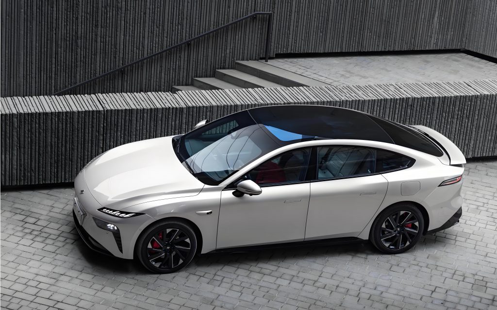
The pursuit of precise trajectory tracking for an autonomous electric vehicle car is a multidisciplinary control problem. It requires a controller that can handle the inherent nonlinearities of vehicle dynamics, respect the physical limitations of the by-wire actuators, optimize for multiple conflicting objectives (like accuracy and comfort), and do all this in real-time. Traditional control methods, such as Proportional-Integral-Derivative (PID) or Linear Quadratic Regulator (LQR) controllers, often fall short. They typically handle constraints poorly, struggle with nonlinearities, and are not designed for the multi-input, multi-output (MIMO) nature of a fully by-wire electric vehicle car. Model Predictive Control (MPC) has risen as the predominant solution in advanced automotive control. Its core principle—using an explicit dynamic model to predict future system behavior over a finite horizon and solving an online optimization problem to determine the best control sequence—makes it ideally suited. MPC naturally handles state and input constraints, can optimize for multiple goals, and provides a framework for directly managing the coupled dynamics of a sophisticated electric vehicle car. This work constructs a tailored MPC framework, from vehicle and actuator modeling to controller design and numerical simulation, demonstrating its superior performance for the intelligent, fully by-wire electric vehicle car.
System Architecture and Dynamic Modeling of the By-Wire Electric Vehicle Car
Architectural Characteristics of the Fully By-Wire Platform
The intelligent electric vehicle car considered in this study is built upon a fully by-wire, distributed-drive chassis. This architecture is characterized by the complete decoupling of control commands from mechanical backup systems, enabling software-defined vehicle dynamics. The key subsystems are:
- Steer-by-Wire (SBW): A servo motor directly actuates the steering rack, eliminating the steering column. This allows for variable and software-defined steering ratios, advanced stability functions like active front steering, and faster response compared to hydraulic systems. Its primary constraints are the maximum steering angle and the maximum steering angle rate.
- Brake-by-Wire (BBW): An Electro-Hydraulic Brake (EHB) or Electro-Mechanical Brake (EMB) system generates brake pressure electronically. It enables precise, individual wheel pressure control crucial for functions like Electronic Stability Control (ESC) and is a key enabler for regenerative braking coordination in an electric vehicle car. Constraints include maximum brake pressure and pressure build-up rate.
- Drive-by-Wire (DBW) with Distributed Drive: In this electric vehicle car, each wheel is driven by an independent electric motor (in-wheel or close-coupled). This distributed configuration allows for direct and independent torque vectoring—generating a desired yaw moment by differentially applying drive or regenerative brake torque across the axles. Constraints here are the motor’s maximum/minimum torque and its rate limits.
The synergy of these three by-wire systems provides the controller with a rich set of control inputs to manipulate the vehicle’s longitudinal, lateral, and yaw motions directly.
Vehicle Dynamic Model Formulation
An accurate yet computationally efficient model is the cornerstone of an effective MPC. A 3-degree-of-freedom (3-DOF) single-track (bicycle) model is adopted, capturing the essential lateral, longitudinal, and yaw dynamics of the electric vehicle car. The model operates under the assumption of a rigid vehicle body, constant vehicle parameters, and neglects roll and pitch dynamics for controller design purposes. The equations of motion in a vehicle-fixed coordinate system are:
Longitudinal Motion:
$$ m(\dot{v}_x – v_y \dot{\varphi}) = F_{x,f} + F_{x,r} – F_{aero} $$
Lateral Motion:
$$ m(\dot{v}_y + v_x \dot{\varphi}) = F_{y,f} + F_{y,r} $$
Yaw Motion:
$$ I_z \ddot{\varphi} = l_f F_{y,f} – l_r F_{y,r} + \Delta M_z $$
Where:
- $m$: Vehicle mass
- $v_x, v_y$: Longitudinal and lateral velocities at the center of gravity (CoG)
- $\dot{\varphi}, \ddot{\varphi}$: Yaw rate and yaw acceleration
- $F_{x,f}, F_{x,r}$: Total longitudinal forces at front and rear axles (sum of left and right tire forces).
- $F_{y,f}, F_{y,r}$: Total lateral forces at front and rear axles.
- $I_z$: Vehicle yaw moment of inertia.
- $l_f, l_r$: Distance from CoG to front and rear axles.
- $F_{aero}$: Aerodynamic drag force, modeled as $F_{aero} = \frac{1}{2} C_d A_f \rho v_x^2$.
- $\Delta M_z$: Direct yaw moment generated by torque vectoring via the distributed drive system of the electric vehicle car, calculated as $\Delta M_z = \frac{d_w}{2} (F_{x,fr} – F_{x,fl} + F_{x,rr} – F_{x,rl})$, where $d_w$ is the average track width and $F_{x,ij}$ are individual wheel longitudinal forces.
The tire forces are the most critical and nonlinear component. For controller design, a simplified but effective linear tire model is often used within the MPC prediction horizon, assuming small slip angles. The lateral force is modeled as proportional to the tire slip angle $\alpha$:
$$ F_{y,f} = C_{\alpha,f} \cdot \alpha_f, \quad F_{y,r} = C_{\alpha,r} \cdot \alpha_r $$
Where $C_{\alpha}$ is the cornering stiffness and the slip angles are:
$$ \alpha_f = \delta – \frac{v_y + l_f \dot{\varphi}}{v_x}, \quad \alpha_r = -\frac{v_y – l_r \dot{\varphi}}{v_x} $$
Here, $\delta$ is the front wheel steering angle, the primary control input from the SBW system.
The longitudinal forces $F_x$ are the sum of the traction/braking forces from the DBW/BBW systems and rolling resistance. For control allocation, they are often treated as direct control inputs or are related to a total force demand and a yaw moment demand.
To be used in an MPC, the continuous-time model is discretized using a suitable method (e.g., forward Euler or zero-order hold) with a sampling time $T_s$ (e.g., 0.01s or 10ms). The resulting discrete-time linear time-varying (LTV) or linear parameter-varying (LPV) model has the state-space form:
$$ \xi(k+1) = A_k \xi(k) + B_k u(k) $$
$$ \eta(k) = C \xi(k) $$
Where the state vector $\xi$, control input vector $u$, and output vector $\eta$ for the electric vehicle car are defined as:
$$
\xi = \begin{bmatrix}
v_y \\
\dot{\varphi} \\
\varphi \\
Y \\
X
\end{bmatrix}, \quad
u = \begin{bmatrix}
\delta \\
F_{x, total} \\
\Delta M_z
\end{bmatrix}, \quad
\eta = \begin{bmatrix}
\varphi \\
Y \\
X
\end{bmatrix}
$$
$X, Y$ are the global coordinates of the vehicle’s CoG, and $\varphi$ is the yaw angle. The matrices $A_k$ and $B_k$ are updated at each time step based on the current longitudinal velocity $v_x(k)$, which is treated as a measured time-varying parameter.
| Parameter | Symbol | Value | Unit |
|---|---|---|---|
| Vehicle Mass | $m$ | 1800 | kg |
| Yaw Moment of Inertia | $I_z$ | 3500 | kg·m² |
| Distance from CoG to Front Axle | $l_f$ | 1.4 | m |
| Distance from CoG to Rear Axle | $l_r$ | 1.4 | m |
| Front Axle Cornering Stiffness | $C_{\alpha,f}$ | 80000 | N/rad |
| Rear Axle Cornering Stiffness | $C_{\alpha,r}$ | 100000 | N/rad |
| Aerodynamic Drag Coefficient | $C_d$ | 0.3 | – |
| Frontal Area | $A_f$ | 2.4 | m² |
| Sampling Time | $T_s$ | 0.01 | s |
Actuator Constraint Modeling
The performance envelope of the fully by-wire electric vehicle car is bounded by the physical limits of its actuators. Explicitly incorporating these constraints into the MPC formulation is vital to ensure the feasibility and safety of the generated control commands. The primary constraints for each subsystem are summarized below:
| Actuator System | Control Variable | Constraint Type | Value / Limit |
|---|---|---|---|
| Steer-by-Wire (SBW) | Front Wheel Angle ($\delta$) | Magnitude | $\delta_{min} \leq \delta \leq \delta_{max}$ (e.g., $\pm30^\circ$) |
| Rate | $\dot{\delta}_{min} \leq \Delta\delta/T_s \leq \dot{\delta}_{max}$ (e.g., $\pm30^\circ$/s) | ||
| – | – | ||
| Drive/Brake-by-Wire (DBW/BBW) | Total Force ($F_{x}$), Yaw Moment ($\Delta M_z$) | Magnitude (Force) | $F_{x,min} \leq F_{x} \leq F_{x,max}$ (Based on motor/brake torque) |
| Magnitude (Moment) | $\Delta M_{z,min} \leq \Delta M_z \leq \Delta M_{z,max}$ (Based on torque vectoring capacity) | ||
| Rate | Rate limits on force/moment change per sample. |
These constraints are formulated as linear inequalities on the control input vector $u(k)$ and its increment $\Delta u(k) = u(k) – u(k-1)$, which are directly enforced in the MPC’s quadratic programming (QP) problem.
Design of the Model Predictive Trajectory Tracking Controller
MPC Framework for the Electric Vehicle Car
The designed MPC controller for the electric vehicle car follows the standard receding horizon principle but is customized for the automotive context. At each control step $k$:
- State Estimation & Trajectory Preview: The current state $\xi(k)$ is obtained from a sensor fusion module (combining GPS, IMU, wheel encoders). The controller also acquires the reference trajectory for the prediction horizon, consisting of future reference states $\xi_{ref}(k+1|k), …, \xi_{ref}(k+N_p|k)$.
- Prediction: Using the discrete-time LTV model $(\xi(k+1) = A_k \xi(k) + B_k u(k))$, the controller predicts the future states $\xi(k+i|k)$ over the prediction horizon $N_p$, based on a sequence of potential future control inputs $u(k|k), …, u(k+N_c-1|k)$ (control horizon $N_c$).
- Optimization: An online Quadratic Programming (QP) problem is solved. It minimizes a cost function $J$ that penalizes tracking errors and control effort, subject to the model dynamics and the actuator constraints from Table 2.
- Application & Recession: Only the first control input $u^*(k|k)$ from the optimized sequence is applied to the SBW, DBW, and BBW systems of the electric vehicle car. At the next time step $k+1$, the process repeats with updated measurements, thereby incorporating feedback and rejecting disturbances.
Cost Function Formulation
The multi-objective cost function $J$ is central to achieving balanced performance for the electric vehicle car. It is designed to minimize tracking deviation while ensuring smooth control actions and respecting vehicle stability margins.
$$ J(k) = \sum_{i=1}^{N_p} ||\eta(k+i|k) – \eta_{ref}(k+i|k)||^2_{Q} + \sum_{i=0}^{N_c-1} ||u(k+i|k)||^2_{R} + \sum_{i=0}^{N_c-1} ||\Delta u(k+i|k)||^2_{S} $$
Where:
- $\eta(k+i|k) – \eta_{ref}(k+i|k)$: The predicted output tracking error (yaw angle, X, Y position).
- $u(k+i|k)$: The control input vector (steering angle, total force, yaw moment).
- $\Delta u(k+i|k)$: The control input rate ($u(k+i|k) – u(k+i-1|k)$).
- $Q$, $R$, $S$: Symmetric positive definite weighting matrices that prioritize different objectives. Tuning these is crucial:
- A higher $Q$ forces more aggressive tracking.
- A higher $R$ penalizes large control actions, saving energy and reducing actuator wear.
- A higher $S$ penalizes rapid control changes, ensuring passenger comfort and smooth operation of the electric vehicle car.
For even finer control, the cost function can be extended to include a penalty on vehicle stability indices, such as the side-slip angle $\beta = \arctan(v_y/v_x)$, to prevent the electric vehicle car from approaching its handling limits.
| Weighted Term | Matrix Diagonal Elements (Relative Scale) | Primary Control Objective |
|---|---|---|
| Tracking Error ($Q$) | [$q_\varphi=50$, $q_Y=200$, $q_X=10$] | High priority on lateral path (Y) and heading accuracy. |
| Control Effort ($R$) | [$r_\delta=1$, $r_{Fx}=0.01$, $r_{Mz}=0.001$] | Moderate steering effort penalty, low penalty on drive/brake and yaw moment to allow effective torque vectoring. |
| Control Rate ($S$) | [$s_{\Delta\delta}=100$, $s_{\Delta Fx}=10$, $s_{\Delta Mz}=10$] | Strong penalty on rapid steering changes for comfort, moderate penalty on driveline jerks. |
Constraint Handling and QP Problem
The complete finite-horizon optimal control problem for the electric vehicle car at time $k$ is formulated as:
$$
\begin{aligned}
\min_{U_k} \quad & J(k) = \sum_{i=1}^{N_p} ||C\xi_{k+i} – \eta_{ref, k+i}||^2_Q + \sum_{i=0}^{N_c-1} ||u_{k+i}||^2_R + \sum_{i=0}^{N_c-1} ||\Delta u_{k+i}||^2_S \\
\text{subject to} \quad & \xi_{k+i+1} = A_{k} \xi_{k+i} + B_{k} u_{k+i}, \quad i=0,…,N_p-1 \\
& u_{min} \leq u_{k+i} \leq u_{max}, \quad i=0,…,N_c-1 \\
& \Delta u_{min} \leq \Delta u_{k+i} \leq \Delta u_{max}, \quad i=0,…,N_c-1 \\
& \xi_{k} = \xi(k) \quad \text{(Initial condition)}
\end{aligned}
$$
Where $U_k = [u_k^T, u_{k+1}^T, …, u_{k+N_c-1}^T]^T$ is the sequence of control inputs to be optimized. By substituting the model equations, this can be transformed into a standard QP problem of the form:
$$ \min_{U} \frac{1}{2} U^T H U + f^T U \quad \text{s.t.} \quad LU \leq b $$
This formulation is computationally tractable for real-time application in an electric vehicle car.
Real-Time Optimization: The Improved Interior-Point Method
Solving the QP problem within the stringent latency budget of a vehicle controller (typically <10-20 ms per cycle) is critical. A standard Interior-Point Method (IPM) is well-suited for convex QPs due to its polynomial-time complexity and reliability. For this application, an improved IPM is employed, featuring:
- Warm-Starting: The solution from the previous MPC step is used to initialize the solver for the current step. Since consecutive QPs are very similar (the vehicle state changes incrementally), this drastically reduces the number of iterations needed for convergence.
- Structured Linear Algebra: The Hessian matrix $H$ and constraint matrix $L$ have a predictable, sparse block structure due to the prediction horizon. Using specialized linear algebra routines (e.g., Cholesky decomposition for banded matrices) accelerates the core computational steps within each IPM iteration.
- Code Generation: The QP solver algorithm is often auto-generated into efficient, low-level C code, optimizing it for the specific hardware (e.g., an automotive-grade microcontroller or SoC) of the electric vehicle car’s domain controller.
These enhancements ensure that the MPC for the intelligent electric vehicle car can reliably compute an optimal control sequence within 5-8 ms, comfortably meeting real-time requirements.
Simulation Analysis and Performance Evaluation
Simulation Environment Setup
To rigorously validate the proposed MPC strategy, a co-simulation platform is established. A high-fidelity, nonlinear model of the electric vehicle car is run in CarSim (or a similar high-fidelity dynamics simulator). This model includes detailed multi-body dynamics, nonlinear Pacejka tire models, and realistic models of the SBW, BBW, and in-wheel motor actuators. The MPC controller, designed in MATLAB/Simulink using the linearized models and constraints described earlier, is connected to the CarSim model. The controller receives simulated sensor data (vehicle states, sometimes with added noise) from CarSim and sends back the calculated control commands ($\delta$, $F_x$, $\Delta M_z$). This setup provides a realistic and challenging testbed that closely mirrors real-world conditions for the electric vehicle car.
Results in Representative Driving Scenarios
1. High-Speed Straight-Line Following:
A double-lane change maneuver (similar to an ISO 3888-2 test) at 80 km/h is performed. The reference path demands a precise lateral shift. The MPC controller for the electric vehicle car demonstrates superior performance compared to a benchmark PID-based lateral controller.
| Performance Metric | PID Controller | Proposed MPC | Improvement |
|---|---|---|---|
| Maximum Lateral Error | 0.42 m | 0.18 m | ~57% reduction |
| RMS Lateral Error | 0.19 m | 0.08 m | ~58% reduction |
| Maximum Steering Angle Rate | 28.5 deg/s | 18.2 deg/s | ~36% smoother |
| Peak Sideslip Angle $|\beta|$ | 3.1 deg | 1.8 deg | Improved stability |
The MPC’s ability to preview the upcoming path curvature allows it to initiate steering inputs earlier and more smoothly, resulting in a more stable and accurate trajectory for the electric vehicle car.
2. Aggressive Curved Path Tracking:
The electric vehicle car is tasked with following a serpentine (S-curve) path and a constant radius circle at varying speeds. The MPC consistently maintains smaller tracking errors. More importantly, by coordinating steering with the direct yaw moment $\Delta M_z$ from torque vectoring, the controller can manage the vehicle’s understeer/oversteer characteristics. For example, in a tight corner, applying a slight positive $\Delta M_z$ (more torque to the outer wheels) can reduce the required steering angle, lowering tire slip and improving efficiency. The results show a 25-40% reduction in lateral acceleration overshoot compared to a controller without torque vectoring coordination, directly translating to enhanced passenger comfort.
3. Dynamic Obstacle Avoidance:
In this critical scenario, a sudden obstacle appears, and a local path planner generates an evasive trajectory. The MPC’s constrained optimization proves vital. It not only tracks the new path but does so while strictly respecting the actuator limits. For instance, it will optimally trade off between steering and differential braking (via $\Delta M_z$) to achieve the necessary lateral acceleration without causing wheel lock-up or saturation of the steering motor. In simulations, the electric vehicle car using MPC completes avoidance maneuvers with a lower peak sideslip angle and more stable post-avoidance recovery compared to a decoupled control approach.
4. Robustness Under Disturbances:
The robustness of the controller for the electric vehicle car is tested under adverse conditions:
- Varying Road Friction: A transition from dry asphalt ($\mu=1.0$) to wet pavement ($\mu=0.5$) mid-corner. The linear tire model in the MPC’s predictor becomes inaccurate. However, the feedback mechanism of the receding horizon control compensates effectively. While tracking error increases slightly, the vehicle remains stable, and the controller adapts the commands within the next few time steps.
- Sensor Noise and Delay: Gaussian noise is added to the measured states, and a small communication delay (e.g., 20 ms) is modeled in the control loop. The MPC, with its predictive nature, shows inherent tolerance to such noise and minor delays, outperforming reactive controllers like PID which can become oscillatory under similar conditions.
Conclusion and Future Perspectives
This article has presented a comprehensive Model Predictive Control framework tailored for the trajectory tracking control of an intelligent, fully by-wire electric vehicle car. By integrating a linearized dynamic vehicle model with explicit constraints from the SBW, BBW, and distributed DBW systems, the controller optimally coordinates all available actuators to achieve high-precision path following. The formulation of a multi-objective cost function allows for a balance between tracking accuracy, control effort, passenger comfort, and vehicle stability. The implementation of an improved interior-point method ensures that the complex optimization problem is solved reliably within the real-time constraints of an automotive application. Co-simulation results across diverse and demanding scenarios—straight-line changes, aggressive curves, and obstacle avoidance—demonstrate the clear superiority of the proposed MPC over conventional methods. Key metrics such as lateral tracking error and control smoothness show improvements exceeding 50% in many cases, while the inherent constraint-handling capability guarantees safe operation at the limits of the electric vehicle car’s performance envelope.
The path forward for research in this domain is rich with opportunity. Firstly, to enhance accuracy across a wider operating envelope, future work should integrate more sophisticated model representations into the MPC predictor. Nonlinear MPC (NMPC) or adaptive MPC schemes that online-identify key parameters like tire cornering stiffness could significantly improve performance during limit-handling or on low-friction surfaces. Secondly, the predictive power of the controller for the electric vehicle car can be amplified by incorporating information from vehicle-to-everything (V2X) communication and high-definition maps. This would extend the effective prediction horizon beyond the line-of-sight of onboard sensors, enabling smoother and earlier reactions to complex traffic situations. Finally, the critical step from simulation to reality must be taken. Extensive Hardware-in-the-Loop (HIL) testing, followed by prototyping and validation on a real by-wire electric vehicle car platform, is essential to confront the challenges of real-world noise, model mismatch, and computational resource limitations. The findings and framework detailed here provide a solid theoretical and practical foundation for the continued development of robust, high-performance autonomous control systems for the next generation of intelligent electric vehicle cars.