
I began this study because the permanent magnet synchronous motor has become one of the most attractive choices for electric vehicle traction, high-speed spindles, and precision drive systems. In my view, the permanent magnet synchronous motor offers precise speed regulation, a high power factor, and low energy consumption, but these advantages are tightly connected to the thermal state of the machine. When the permanent magnet synchronous motor operates at high speed, electromagnetic loss, copper loss, iron loss, and eddy-current loss generate heat inside the stator, rotor, winding, and permanent magnets. If I ignore that heat, I cannot correctly predict torque, efficiency, demagnetization margin, or lifetime. Therefore, I developed an improved multi-objective nonlinear magnetic-thermal coupling iterative calculation method for a permanent magnet synchronous motor and then used it to optimize the cooling channel layout.
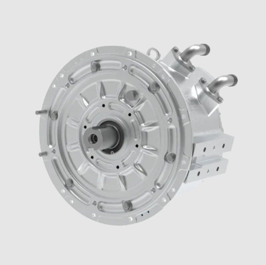
My central argument is simple: a permanent magnet synchronous motor is not a purely electromagnetic device and not a purely thermal device. It is a coupled system. The electrical resistivity of copper increases with temperature, the residual flux density and coercivity of the permanent magnet change with temperature, and high temperature can push the permanent magnet toward irreversible demagnetization. At the same time, demagnetization changes the air-gap flux density, the back electromotive force, the current waveform, and the loss distribution. In my improved method, I iterate between a two-dimensional transient electromagnetic model and a three-dimensional global heat-transfer model until both the permanent magnet average temperature and the stator winding average temperature converge. I then use orthogonal experiments to study how channel number, coolant inlet flow rate, cooling medium, and inlet/outlet arrangement angle affect the thermal field and pressure drop of the permanent magnet synchronous motor.
1. Motivation and Scope
I selected a 40 kW automotive permanent magnet synchronous motor as my reference machine. The machine has an 8-pole, 48-slot configuration, a double-layer winding, and an interior permanent magnet rotor. The rated operating point is 40 kW at 8100 r/min with 48 N·m, and a second high-speed operating point is 40 kW at 12000 r/min with 32 N·m. I use these two operating points because they represent different thermal and electromagnetic stress patterns. The first point has higher torque and higher copper loss, while the second point has higher frequency and higher iron loss. For a permanent magnet synchronous motor used in a vehicle, both points matter because the driver may demand maximum torque at low speed or sustained power at high speed.
In my analysis, I do not treat loss as a fixed input. Instead, I calculate the electromagnetic field, extract the loss density in each region, transfer that loss to the thermal model, obtain the temperature distribution, update the material properties, and recalculate the electromagnetic field. This loop is the core of my improved multi-objective nonlinear magnetic-thermal coupling method. I call it multi-objective because I monitor two separate convergence targets: the average temperature of the permanent magnet and the average temperature of the stator winding. I call it nonlinear because I include the nonlinear B-H behavior of the permanent magnet and the magnetic saturation of the stator and rotor laminations. I call it magnetic-thermal coupling because the electromagnetic field and the temperature field influence each other rather than being solved in only one direction.
2. Reference Machine and Physical Parameters
I first fixed the main dimensions and rated data of the permanent magnet synchronous motor. The values I used are listed in Table 1. These parameters define the electromagnetic model, the thermal model, and the cooling jacket geometry. I kept the stator outer diameter and axial length compatible with an automotive traction application, and I kept the air gap small enough to achieve high torque density while still allowing a realistic manufacturing tolerance.
| Parameter | Value |
|---|---|
| Rated power | 40 kW |
| Rated speed | 8100 r/min |
| Rated torque | 48 N·m |
| Peak speed | 12000 r/min |
| Peak torque at high speed | 32 N·m |
| Stator outer diameter | 180 mm |
| Stator inner diameter | 120 mm |
| Air gap | 0.6 mm |
| Number of poles | 8 |
| Number of slots | 48 |
| Winding type | Double-layer |
| Rotor type | Interior permanent magnet |
For the electromagnetic calculation, I exploited the periodic symmetry of the permanent magnet synchronous motor and solved a one-eighth model. This reduced the computational cost while preserving the field distribution in one pole pair. I used a transient solver because the permanent magnet synchronous motor operates with time-varying current, rotating rotor position, and moving magnetic field. The mesh in the air gap was refined to capture slotting effects and flux leakage around the magnetic bridges. The mesh in the permanent magnet and stator teeth was also refined because these regions determine the loss and saturation behavior.
From the no-load electromagnetic solution, I observed that the flux density was distributed in a periodic and balanced way. The highest flux density appeared near the rotor magnetic bridges and the inner edges of the permanent magnet pockets. This is expected in an interior permanent magnet synchronous motor because the bridges act as mechanical supports and also as magnetic leakage paths. The air-gap flux density was approximately sinusoidal, with a peak near 0.8 T. The Fourier decomposition showed that the fundamental component dominated, and the higher-order harmonics were limited. I considered this acceptable for the permanent magnet synchronous motor because excessive harmonics would increase iron loss, torque ripple, and acoustic noise.
3. Electromagnetic Field Model
I used the standard transient magnetic field formulation for the permanent magnet synchronous motor. In the two-dimensional plane, the governing equation for the magnetic vector potential can be written as
$$ \frac{\partial}{\partial x}\left(\nu \frac{\partial A_z}{\partial x}\right)+\frac{\partial}{\partial y}\left(\nu \frac{\partial A_z}{\partial y}\right) = -J_z + \sigma \frac{\partial A_z}{\partial t} $$
where \(A_z\) is the magnetic vector potential in the axial direction, \(\nu\) is the magnetic reluctivity, \(J_z\) is the applied current density, and \(\sigma\) is the electrical conductivity. For the permanent magnet regions, I added the equivalent current sheet or the coercive force term to represent the magnetomotive force of the permanent magnet. In the rotor and stator laminations, I used a nonlinear B-H curve to represent magnetic saturation. In the permanent magnet, I used a temperature-dependent demagnetization curve because the permanent magnet synchronous motor can experience significant temperature rise under continuous load.
The electromagnetic torque of the permanent magnet synchronous motor is computed from the magnetic field solution. In the dq reference frame, I can express the torque as
$$ T_e = \frac{3}{2} p \left(\psi_d i_q – \psi_q i_d\right) $$
where \(p\) is the pole pair number, \(\psi_d\) and \(\psi_q\) are the d-axis and q-axis flux linkages, and \(i_d\) and \(i_q\) are the d-axis and q-axis currents. The mechanical output power is
$$ P_{out} = T_e \omega_m $$
where \(\omega_m\) is the mechanical angular speed. I used these equations to check that the permanent magnet synchronous motor met the required torque and power at both operating points. The torque curves were stable, and the power curves followed the intended constant-power region at high speed. This confirmed that the electromagnetic design was reasonable before I moved to the thermal problem.
I also examined the flux-weakening capability of the permanent magnet synchronous motor. At 12000 r/min, the back electromotive force increases, so the controller must apply negative d-axis current to weaken the air-gap flux. This current increases copper loss and can also increase permanent magnet eddy-current loss because the harmonic content of the air-gap field changes. In my magnetic-thermal coupling method, I therefore include the high-speed operating point as a separate case. I do not assume that the rated torque point is always the worst thermal case. For a permanent magnet synchronous motor, the high-speed point can be thermally critical because iron loss and magnet eddy loss increase with frequency, even if the torque is lower.
4. Loss Calculation
I calculated four loss components: stator iron loss, rotor iron loss, permanent magnet eddy-current loss, and winding copper loss. I deliberately excluded mechanical friction and windage loss from the thermal source because their contribution is small compared with electromagnetic loss in this permanent magnet synchronous motor, and because the cooling jacket mainly removes stator and winding heat. The iron loss was calculated using the Bertotti model:
$$ P_{Fe} = k_h f B_m^\alpha + k_e f^2 B_m^2 + k_a f^{1.5} B_m^{1.5} $$
where \(B_m\) is the peak magnetic flux density, \(f\) is the electrical frequency, and \(k_h\), \(k_e\), and \(k_a\) are the hysteresis, eddy-current, and excess loss coefficients. I obtained these coefficients by fitting the lamination loss data provided by the steel manufacturer. The frequency \(f\) depends on the rotor speed and the pole pair number:
$$ f = \frac{p n}{60} $$
where \(n\) is the mechanical speed in r/min. For the 8-pole permanent magnet synchronous motor, the electrical frequency at 8100 r/min is 540 Hz, and at 12000 r/min it is 800 Hz. This difference explains why the high-speed operating point has higher iron loss despite lower torque.
The permanent magnet eddy-current loss was calculated from the induced eddy currents in the magnet segments:
$$ P_E = \int_V \mathbf{E}\cdot\mathbf{J}_w \, dV = \int_V \frac{J_w^2}{\sigma} \, dV = \int_V \rho J_w^2 \, dV $$
where \(\mathbf{E}\) is the induced electric field, \(\mathbf{J}_w\) is the eddy-current density, \(\rho\) is the magnet resistivity, \(\sigma\) is the magnet conductivity, and \(V\) is the permanent magnet volume. In a permanent magnet synchronous motor, magnet eddy loss is often smaller than copper loss, but it can still be important because it heats the permanent magnet directly and reduces the demagnetization margin.
The winding copper loss was calculated with temperature dependence:
$$ P_{cu} = m I^2 R $$
$$ R = R_0 \left[1+\beta_0(T-T_0)\right] = \frac{\rho_{za} L_z}{S}\left[1+\beta_0(T-T_0)\right] $$
where \(m\) is the number of phases, \(I\) is the root-mean-square phase current, \(R_0\) is the reference resistance, \(\beta_0\) is the temperature coefficient of copper, \(T_0\) is the reference temperature, \(\rho_{za}\) is the copper resistivity, \(L_z\) is the conductor length, and \(S\) is the conductor cross-sectional area. Because copper resistivity increases with temperature, the copper loss in the permanent magnet synchronous motor increases as the winding heats up. This is one of the main reasons I use an iterative magnetic-thermal coupling method instead of a one-way method.
Table 2 shows the loss values I obtained for the two operating points. The stator iron loss and winding copper loss are the dominant heat sources. The rotor iron loss and permanent magnet eddy loss are smaller in absolute value, but they are located in thermally sensitive regions. In particular, the permanent magnet eddy loss directly affects the permanent magnet temperature and therefore the demagnetization risk of the permanent magnet synchronous motor.
| Operating point | Stator iron loss / W | Rotor iron loss / W | Magnet eddy loss / W | Winding copper loss / W |
|---|---|---|---|---|
| 40 kW, 8100 r/min, 48 N·m | 649.5 | 69.43 | 5.90 | 840 |
| 40 kW, 12000 r/min, 32 N·m | 848.8 | 84.71 | 4.55 | 740 |
After calculating the total loss in each region, I converted the loss into a volumetric heat source. For a region with loss \(Q\), effective heat-transfer area \(A\), and axial length \(L\), the equivalent heat flux is
$$ J = \frac{Q}{A L} $$
I used this heat flux to load the three-dimensional thermal model. In my improved method, the heat flux is not fixed during the entire calculation. It is updated after each electromagnetic solution because the copper resistivity and permanent magnet properties change with temperature. This feedback is what makes the method a true magnetic-thermal coupling method rather than a sequential loss-to-temperature calculation.
5. Improved Multi-Objective Nonlinear Magnetic-Thermal Coupling
Traditional magnetic-thermal coupling for a permanent magnet synchronous motor often considers only the temperature dependence of copper resistivity. In that approach, the permanent magnet is assumed to have a constant B-H curve or a constant recoil permeability, and the demagnetization effect of high temperature is ignored. I found this insufficient for an automotive permanent magnet synchronous motor because the permanent magnet can reach temperatures above 100 °C under continuous operation. At those temperatures, the residual flux density and intrinsic coercivity decrease, and the knee point of the demagnetization curve moves toward the operating point. If the operating point crosses the knee, irreversible demagnetization occurs, and the permanent magnet synchronous motor loses torque capability.
To include this physics, I used temperature-dependent expressions for the permanent magnet:
$$ B_{r,t1} = \left(1-\frac{IL}{100}\right)\left[1+\frac{(t_1-t_0)\alpha_{Br}}{100}\right] B_{r,t0} $$
$$ H_{c,t1} = \left(1-\frac{IL}{100}\right)\left[1+\frac{(t_1-t_0)\alpha_{Hc}}{100}\right] H_{c,t0} $$
where \(B_{r,t0}\) is the residual flux density at the reference temperature \(t_0\), \(H_{c,t0}\) is the coercivity at the reference temperature, \(\alpha_{Br}\) is the reversible temperature coefficient of residual flux density, \(\alpha_{Hc}\) is the temperature coefficient of coercivity, and \(IL\) is the irreversible loss percentage. In my calculation, I set the irreversible loss to zero during normal operation and used the reversible temperature coefficients to shift the demagnetization curve. I then checked the minimum operating point on the demagnetization curve to ensure that the permanent magnet synchronous motor retained an adequate margin.
For the copper winding, I used the temperature-dependent resistivity:
$$ \rho = \rho_0 \left[1+\beta_0(T-T_0)\right] $$
where \(\rho_0\) is the reference resistivity and \(\beta_0\) is the temperature coefficient. This changes the copper loss and therefore changes the heat generation in the winding. Because the winding is one of the hottest parts of the permanent magnet synchronous motor, this feedback is essential for accurate temperature prediction.
I defined two convergence criteria, one for the permanent magnet and one for the stator winding:
$$ \left|\frac{T_{pa}^{n+1}-T_{pa}^{n}}{T_{pa}^{n+1}}\right| \le \epsilon_1 $$
$$ \left|\frac{T_{za}^{n+1}-T_{za}^{n}}{T_{za}^{n+1}}\right| \le \epsilon_2 $$
where \(T_{pa}^{n}\) is the average permanent magnet temperature at iteration \(n\), \(T_{za}^{n}\) is the average stator winding temperature at iteration \(n\), and \(\epsilon_1\) and \(\epsilon_2\) are the convergence tolerances. I set both tolerances to 0.8%. In practice, I required both criteria to be satisfied at the same iteration before I accepted the result. This prevents a situation in which the winding temperature has converged but the permanent magnet temperature is still drifting, or vice versa.
Because commercial magnet data are usually available only at discrete temperatures such as 80 °C, 100 °C, and 120 °C, I used linear interpolation to estimate the demagnetization curve at intermediate temperatures. The interpolation formula I used is
$$ \psi(B,H) = \frac{f_{x1}(B,H)-f_{x0}(B,H)}{x_1-x_0} $$
$$ f_x(B,H) = f_{x0}(B,H) + \psi(B,H)(x-x_0) $$
where \(f_{x0}(B,H)\) and \(f_{x1}(B,H)\) are the demagnetization curves at the known temperatures \(x_0\) and \(x_1\), and \(f_x(B,H)\) is the interpolated curve at temperature \(x\). This allowed me to update the permanent magnet B-H curve at every iteration without requiring a full thermal demagnetization dataset.
Table 3 shows the key parameter evolution for the traditional magnetic-thermal coupling method. Table 4 shows the key parameter evolution for my improved multi-objective nonlinear magnetic-thermal coupling method. In the traditional method, only the copper resistivity is updated, and the permanent magnet curve remains fixed. In my improved method, both the copper resistivity and the permanent magnet B-H curve are updated. The improved method required more iterations, but it produced a more realistic temperature distribution and a more reliable demagnetization assessment.
| Operating point | Iteration | Initial temperature / °C | \(\rho_{za}^{n+1}\) / (Ω/m) | Average winding temperature / °C | Maximum winding temperature / °C | Relative change / % |
|---|---|---|---|---|---|---|
| 40 kW, 8100 r/min, 48 N·m | 1 | 80 | 2.19 | 107.77 | 109.52 | — |
| 2 | 107.77 | 2.384 | 109.57 | 111.39 | 1.60 | |
| 3 | 109.57 | 2.396 | 110.47 | 112.32 | 0.81 | |
| 4 | 110.47 | 2.403 | 110.69 | 112.55 | 0.19 | |
| 40 kW, 12000 r/min, 32 N·m | 1 | 80 | 2.19 | 105.17 | 106.86 | — |
| 2 | 105.17 | 2.366 | 106.97 | 108.72 | 1.62 | |
| 3 | 106.97 | 2.378 | 107.87 | 109.66 | 0.84 | |
| 4 | 107.87 | 2.385 | 108.09 | 109.89 | 0.20 |
| Operating point | Iteration | Permanent magnet B-H temperature / °C | \(\rho_{za}^{n+1}\) / (Ω/m) | Average permanent magnet temperature / °C | Maximum permanent magnet temperature / °C | Average winding temperature / °C | Maximum winding temperature / °C | Relative change / % |
|---|---|---|---|---|---|---|---|---|
| 40 kW, 8100 r/min, 48 N·m | 1 | 80 | 2.19 | 93.31 | 94.42 | 109.0 | 110.75 | — |
| 2 | 93 | 2.393 | 100.1 | 101.7 | 117.0 | 120.04 | 6.78 / 6.83 | |
| 3 | 100 | 2.449 | 104.3 | 105.8 | 121.21 | 122.95 | 4.02 / 3.47 | |
| 4 | 104 | 2.477 | 103.94 | 106.60 | 122.02 | 124.80 | 0.34 / 0.66 | |
| 5 | 104 | 2.484 | 104.42 | 106.0 | 122.44 | 124.82 | 0.45 / 0.34 | |
| 40 kW, 12000 r/min, 32 N·m | 1 | 80 | 2.19 | 97.24 | 98.46 | 106.56 | 108.32 | — |
| 2 | 97 | 2.376 | 104.56 | 106.05 | 115.21 | 117.33 | 7.00 / 7.50 | |
| 3 | 104 | 2.436 | 108.56 | 109.89 | 118.02 | 121.02 | 3.68 / 2.38 | |
| 4 | 108 | 2.456 | 109.3 | 112.5 | 117.0 | 119.5 | 0.67 / 0.87 | |
| 5 | 109 | 2.449 | 108.79 | 110.43 | 117.29 | 119.51 | 0.46 / 0.24 |
I observed that the improved method converged to a higher winding temperature than the traditional method. This is expected because the improved method accounts for the increased copper loss caused by higher temperature and the reduced permanent magnet flux caused by high temperature. The reduced permanent magnet flux requires slightly more current to produce the same torque, which further increases copper loss. This positive feedback is exactly the kind of behavior that a permanent magnet synchronous motor exhibits in real operation. If I neglect it, I underpredict the winding temperature and overestimate the demagnetization margin.
6. Thermal Model and Boundary Conditions
For the thermal analysis, I built a three-dimensional global heat-transfer model of the permanent magnet synchronous motor. The model includes the housing, cooling jacket, stator, rotor, shaft, winding, slot insulation, air gap, and permanent magnets. I used a polyhedral mesh in the fluid region and a hexahedral-dominant mesh in the solid region. The mesh was refined near the cooling channel walls, the slot liner, the permanent magnet surfaces, and the air gap. I included the thermal contact resistance between the laminations and the housing, and I represented the slot insulation as a separate solid layer.
The cooling jacket uses an external water-cooling arrangement. The inlet water temperature was set to 65 °C, and the inlet flow rate was 12 L/min for the baseline case. At the inlet, I applied a velocity boundary condition. At the outlet, I applied a pressure boundary condition. The outer surface of the housing exchanges heat with ambient air through natural convection. The shaft ends also exchange heat with air. The air gap was modeled as a thin fluid region with effective thermal conductivity to account for the rotating flow and the small clearance.
The material properties I used are listed in Table 5. The stator and rotor laminations are orthotropic because the laminated core has different thermal conductivity in the radial and axial directions. The winding is represented as a homogeneous copper region with equivalent insulation properties. The permanent magnet has a relatively low thermal conductivity compared with copper, so heat removal from the magnet is slower. This is one reason the permanent magnet temperature can remain high even when the housing is well cooled.
| Material | Density / (kg/m³) | Specific heat / [J/(kg·K)] | Thermal conductivity / [W/(m·K)] |
|---|---|---|---|
| Housing | 2680 | 963 | 150 |
| Shaft | 7850 | 460 | 48 |
| Slot insulation | 8030 | 502.48 | 0.22 |
| Winding | 8978 | 390 | 401 |
| Stator and rotor core, radial | 8030 | 502.48 | 39 |
| Stator and rotor core, axial | 8030 | 502.48 | 4.43 |
| Coolant | 1073.3 | 3281 | 0.38 |
| Permanent magnet | 8030 | 502.48 | 9 |
I used the improved multi-objective nonlinear magnetic-thermal coupling method to compute the temperature field at both operating points. The temperature distributions showed that the winding was the hottest component, followed by the permanent magnet, the stator core, the rotor core, and the housing. The highest winding temperature occurred near the end winding and in the slot portion close to the air gap. The highest permanent magnet temperature occurred near the rotor surface and near the edges of the magnet pockets. These locations match the loss distribution and the heat-transfer paths. The end winding has poor contact with the stator core, so heat must pass through a long insulation path before reaching the cooling jacket. The permanent magnet is surrounded by rotor iron and air, so heat removal is slower than in the stator.
Table 6 summarizes the maximum and average temperatures I obtained with the improved method. At 8100 r/min and 48 N·m, the average permanent magnet temperature was 104.42 °C, the maximum permanent magnet temperature was 106.0 °C, the average winding temperature was 122.44 °C, and the maximum winding temperature was 124.82 °C. At 12000 r/min and 32 N·m, the average permanent magnet temperature was 108.79 °C, the maximum permanent magnet temperature was 110.43 °C, the average winding temperature was 117.29 °C, and the maximum winding temperature was 119.51 °C. The high-speed point had a higher permanent magnet temperature because the magnet eddy loss and rotor iron loss are concentrated in the rotor, while the lower-speed point had a higher winding temperature because the copper loss is higher.
| Operating point | Component | Average temperature / °C | Maximum temperature / °C |
|---|---|---|---|
| 40 kW, 8100 r/min, 48 N·m | Permanent magnet | 104.42 | 106.0 |
| Stator winding | 122.44 | 124.82 | |
| 40 kW, 12000 r/min, 32 N·m | Permanent magnet | 108.79 | 110.43 |
| Stator winding | 117.29 | 119.51 |
7. Experimental Validation
To validate my method, I compared the computed winding temperatures with measurements from a prototype permanent magnet synchronous motor. The prototype was assembled and tested on a dynamometer. I installed temperature sensors near the end winding and inside the terminal box. I recorded the speed, torque, current, voltage, and resistance over a two-hour period until the winding resistance stabilized. The stabilized temperature was taken as the steady-state winding temperature. I used the same cooling conditions as in the simulation: inlet coolant temperature 65 °C, flow rate 12 L/min, and the same housing geometry.
Table 7 compares the measured winding temperature with the traditional magnetic-thermal coupling result and my improved multi-objective nonlinear magnetic-thermal coupling result. At 8100 r/min and 48 N·m, the measured maximum winding temperature was 120 °C. The traditional method predicted 112.55 °C, an error of 6.2%. My improved method predicted 124.8 °C, an error of 4.0%. At 12000 r/min and 32 N·m, the measured maximum winding temperature was 116 °C. The traditional method predicted 109.89 °C, an error of 5.3%. My improved method predicted 119.5 °C, an error of 3.0%. In both cases, my improved method reduced the error to less than 5%, which I consider acceptable for a coupled electromagnetic-thermal simulation of a permanent magnet synchronous motor.
| Operating point | Measured winding maximum / °C | Traditional coupling / °C | Traditional error / % | Improved nonlinear coupling / °C | Improved error / % |
|---|---|---|---|---|---|
| 40 kW, 8100 r/min, 48 N·m | 120 | 112.55 | 6.2 | 124.8 | 4.0 |
| 40 kW, 12000 r/min, 32 N·m | 116 | 109.89 | 5.3 | 119.5 | 3.0 |
The experimental validation confirms that the temperature dependence of the permanent magnet and the nonlinear B-H behavior cannot be ignored in a permanent magnet synchronous motor. The traditional method underestimates the winding temperature because it does not capture the additional copper loss caused by the higher temperature and the additional current required by the demagnetized permanent magnet. My improved method captures both effects, so it provides a more conservative and more accurate thermal prediction. This is important for designing the cooling system and for setting the current limit of the permanent magnet synchronous motor.
8. Cooling Channel Types
After validating the thermal model, I used it to compare three cooling channel types: spiral, circumferential, and axial Z-shaped. I kept the cross-sectional area of the channel constant and used the same inlet conditions. The spiral channel follows a helical path around the housing. It has the lowest pressure drop because it has no sharp right-angle turns, but its cooling performance is the weakest. The circumferential channel follows a circumferential path with axial connections. It provides a good balance between heat transfer and pressure drop. The axial Z-shaped channel forces the coolant to pass back and forth along the axial direction. It has the best cooling performance because it increases the flow velocity near the hot spots and promotes turbulence, but it also has the highest pressure drop because of multiple right-angle turns.
| Channel type | Cooling performance | Pressure drop | Manufacturing complexity | My assessment |
|---|---|---|---|---|
| Spiral | Lowest | Lowest | Moderate | Not suitable for high power density |
| Circumferential | Medium | Medium | Low to moderate | Best overall compromise |
| Axial Z-shaped | Highest | Highest | High | Good cooling but high pump cost |
At a flow rate of 12 L/min, the circumferential channel produced a maximum temperature of 124.6 °C and a pressure drop of 55.75 kPa. The axial Z-shaped channel produced a lower maximum temperature but a much higher pressure drop. The spiral channel produced the lowest pressure drop but the highest maximum temperature. Considering the cooling effect, the pressure drop, and the manufacturing cost, I selected the circumferential channel as the baseline for further optimization. This choice gives the permanent magnet synchronous motor a robust thermal margin without imposing an excessive hydraulic load on the coolant pump.
9. Orthogonal Experiment Design
I then designed a four-factor, three-level orthogonal experiment to optimize the circumferential channel of the permanent magnet synchronous motor. The four factors are channel number, coolant inlet flow rate, ethylene glycol concentration, and inlet/outlet arrangement angle. I selected these factors because my single-factor studies showed that they influence the maximum temperature and pressure drop to different degrees. Channel number changes the heat-transfer area and the flow velocity. Coolant flow rate changes the convective heat-transfer coefficient and the residence time. Ethylene glycol concentration changes the thermal conductivity, specific heat, viscosity, and freezing point of the coolant. Inlet/outlet arrangement angle changes the flow distribution and the local pressure loss.
I used three levels for each factor. The channel number levels were 3, 4, and 5. The coolant inlet flow rate levels were 4, 10, and 16 L/min. The ethylene glycol concentration levels were 40%, 50%, and 60%. The inlet/outlet arrangement angle levels were 30°, 60°, and 90°. I labeled the factors A, B, C, and D. Table 8 shows the factor-level coding. Table 9 shows the orthogonal experiment plan and the computed maximum temperature and pressure drop for each run. I used the improved multi-objective nonlinear magnetic-thermal coupling method for every run, so the electromagnetic loss and the temperature field were consistent with the thermal state of the permanent magnet synchronous motor.
| Level | A: Channel number | B: Coolant inlet flow / (L/min) | C: Ethylene glycol concentration / % | D: Inlet/outlet angle / (°) |
|---|---|---|---|---|
| 1 | 3 | 4 | 40 | 30 |
| 2 | 4 | 10 | 50 | 60 |
| 3 | 5 | 16 | 60 | 90 |
| Run | A | B | C | D | Maximum motor temperature / °C | Channel pressure drop / kPa |
|---|---|---|---|---|---|---|
| 1 | 1 | 1 | 1 | 1 | 126.91 | 4.39 |
| 2 | 1 | 2 | 2 | 2 | 125.24 | 21.71 |
| 3 | 1 | 3 | 3 | 3 | 124.65 | 57.65 |
| 4 | 2 | 1 | 2 | 3 | 125.90 | 13.38 |
| 5 | 2 | 2 | 3 | 1 | 124.33 | 56.76 |
| 6 | 2 | 3 | 1 | 2 | 123.98 | 91.52 |
| 7 | 3 | 1 | 3 | 2 | 126.51 | 26.23 |
| 8 | 3 | 2 | 1 | 3 | 125.33 | 75.11 |
| 9 | 3 | 3 | 2 | 1 | 124.30 | 165.36 |
10. Range Analysis
I performed range analysis to identify the influence order of each factor. For a factor \(j\), the range is
$$ R_j = \max(\bar{K}_{ij}) – \min(\bar{K}_{ij}) $$
where \(\bar{K}_{ij}\) is the average result for level \(i\) of factor \(j\). A larger range means that the factor has a stronger effect on the response. Table 10 shows the range analysis for the maximum motor temperature. The influence order is B > A > C > D. The coolant inlet flow rate has the largest effect, followed by the channel number, then the ethylene glycol concentration, and finally the inlet/outlet angle. The best level combination for minimizing the maximum temperature is A2B3C2D1, which means 4 channels, 16 L/min, 50% ethylene glycol, and 30° inlet/outlet angle.
| Response | Statistic | A: Channel number | B: Coolant inlet flow / (L/min) | C: Ethylene glycol concentration / % | D: Inlet/outlet angle / (°) |
|---|---|---|---|---|---|
| Maximum motor temperature / °C | K1 | 125.60 | 126.44 | 125.41 | 125.18 |
| K2 | 124.74 | 124.97 | 125.15 | 125.24 | |
| K3 | 125.38 | 124.31 | 125.16 | 125.29 | |
| Range \(R\) | 0.86 | 2.13 | 0.26 | 0.11 | |
| Best level | A2 | B3 | C2 | D1 |
Table 11 shows the range analysis for the channel pressure drop. The influence order is B > A > D > C. Again, the coolant inlet flow rate has the largest effect. The channel number is second, the inlet/outlet angle is third, and the ethylene glycol concentration is fourth. The best level combination for minimizing the pressure drop is A1B1C3D2, which means 3 channels, 4 L/min, 60% ethylene glycol, and 60° inlet/outlet angle. This combination is different from the best combination for temperature, so I needed a multi-objective compromise.
| Response | Statistic | A: Channel number | B: Coolant inlet flow / (L/min) | C: Ethylene glycol concentration / % | D: Inlet/outlet angle / (°) |
|---|---|---|---|---|---|
| Channel pressure drop / kPa | K1 | 27.92 | 14.67 | 57.01 | 75.50 |
| K2 | 53.89 | 51.19 | 66.82 | 46.49 | |
| K3 | 88.90 | 104.84 | 46.88 | 48.71 | |
| Range \(R\) | 60.98 | 90.17 | 19.94 | 29.01 | |
| Best level | A1 | B1 | C3 | D2 |
11. Weighted Multi-Objective Optimization
Because the best temperature combination and the best pressure-drop combination are not the same, I used a weighted scoring method. I normalized both responses so that a smaller value is better. The normalization formula is
$$ X^* = \frac{X_{max}-X}{X_{max}-X_{min}}\times 100 $$
where \(X_{max}\) and \(X_{min}\) are the maximum and minimum values of the response, and \(X\) is the actual value. I assigned equal weights to the maximum temperature and the pressure drop because both are important for the permanent magnet synchronous motor. The weighted score is
$$ S = w_T X_T^* + w_P X_P^* $$
where \(w_T = 0.5\) and \(w_P = 0.5\). A higher score means a better overall result. Table 12 shows the weighted scores for the nine orthogonal runs. Table 13 shows the range analysis of the weighted score. The influence order for the weighted score is A > B > D > C. The channel number has the largest effect on the combined objective, followed by the coolant inlet flow rate, then the inlet/outlet angle, and finally the ethylene glycol concentration.
| Run | A | B | C | D | Maximum temperature / °C | Pressure drop / kPa | Weighted score |
|---|---|---|---|---|---|---|---|
| 1 | 1 | 1 | 1 | 1 | 126.91 | 4.39 | 50.00 |
| 2 | 1 | 2 | 2 | 2 | 125.24 | 21.71 | 73.12 |
| 3 | 1 | 3 | 3 | 3 | 124.65 | 57.65 | 72.02 |
| 4 | 2 | 1 | 2 | 3 | 125.90 | 13.38 | 64.44 |
| 5 | 2 | 2 | 3 | 1 | 124.33 | 56.76 | 77.76 |
| 6 | 2 | 3 | 1 | 2 | 123.98 | 91.52 | 72.94 |
| 7 | 3 | 1 | 3 | 2 | 126.51 | 26.23 | 50.04 |
| 8 | 3 | 2 | 1 | 3 | 125.33 | 75.11 | 55.00 |
| 9 | 3 | 3 | 2 | 1 | 124.30 | 165.36 | 44.54 |
| Statistic | A: Channel number | B: Coolant inlet flow / (L/min) | C: Ethylene glycol concentration / % | D: Inlet/outlet angle / (°) |
|---|---|---|---|---|
| K1 | 65.05 | 54.83 | 59.31 | 57.43 |
| K2 | 71.71 | 68.63 | 60.70 | 65.37 |
| K3 | 49.86 | 63.17 | 66.61 | 63.82 |
| Range \(R\) | 21.85 | 13.80 | 7.29 | 7.93 |
From the weighted score analysis, the best combination is A2B2C3D2. This means 4 channels, a coolant inlet flow rate of 10 L/min, an ethylene glycol concentration of 60%, and an inlet/outlet arrangement angle of 60°. I selected this combination as my optimized cooling design for the permanent magnet synchronous motor. It does not produce the absolute lowest temperature or the absolute lowest pressure drop, but it provides the best compromise between thermal performance and hydraulic loss.
12. Optimized Cooling Performance
After selecting the optimized combination, I re-ran the full multi-objective nonlinear magnetic-thermal coupling simulation. The maximum winding temperature was 124.3 °C, and the channel pressure drop was 50.25 kPa. Compared with the unoptimized circumferential channel at 12 L/min, which had a maximum temperature of 124.6 °C and a pressure drop of 55.75 kPa, the optimized design reduced the maximum temperature by 0.3 °C and reduced the pressure drop by 5.5 kPa. The temperature reduction is modest, but the pressure-drop reduction is significant. In a permanent magnet synchronous motor for an electric vehicle, a lower pressure drop means a smaller pump power requirement and a lower parasitic loss. The optimized channel also distributes the coolant more evenly around the housing, which reduces the local hot spots in the end winding and the permanent magnet.
| Design | Channel number | Flow / (L/min) | Ethylene glycol / % | Inlet/outlet angle / (°) | Maximum temperature / °C | Pressure drop / kPa |
|---|---|---|---|---|---|---|
| Baseline circumferential | 4 | 12 | 50 | 60 | 124.6 | 55.75 |
| Optimized A2B2C3D2 | 4 | 10 | 60 | 60 | 124.3 | 50.25 |
| Improvement | — | −2 | +10 | 0 | −0.3 | −5.5 |
I also compared the optimized design with the other orthogonal runs. The optimized combination had a higher weighted score than any of the nine experimental runs because it balanced temperature and pressure drop. The run with the lowest temperature used 16 L/min and had a pressure drop of 91.52 kPa, which is too high for a practical automotive cooling loop. The run with the lowest pressure drop used 4 L/min and had a maximum temperature of 126.91 °C, which is too high for the permanent magnet synchronous motor. My optimized design avoids both extremes.
13. Thermal-Electromagnetic Feedback in the Optimized Design
One important result of my study is that the optimized cooling design changes the electromagnetic state of the permanent magnet synchronous motor. When the winding and permanent magnet run cooler, the copper resistivity is lower, so the copper loss is lower. The permanent magnet flux density is higher, so less current is needed to produce the same torque. This reduces the current density in the winding and further reduces the loss. Conversely, if the cooling design is poor, the temperature rises, the copper loss increases, and the permanent magnet flux decreases. The controller must then increase the current to maintain torque, which increases loss again. This positive feedback loop is a key feature of the permanent magnet synchronous motor, and it is why my improved multi-objective nonlinear magnetic-thermal coupling method is necessary.
In my optimized design, the permanent magnet average temperature at the rated torque point was 104.42 °C, and the winding average temperature was 122.44 °C. At the high-speed point, the permanent magnet average temperature was 108.79 °C, and the winding average temperature was 117.29 °C. These temperatures are below the irreversible demagnetization threshold of the selected permanent magnet. I also checked the knee point of the demagnetization curve at the highest permanent magnet temperature. The minimum operating flux density remained above the knee, so the permanent magnet synchronous motor retained an adequate margin against irreversible demagnetization.
14. Practical Design Guidelines
From my analysis, I can state several practical guidelines for the thermal design of a permanent magnet synchronous motor. First, the coolant inlet flow rate is the most influential single factor for both maximum temperature and pressure drop. Increasing the flow rate reduces the temperature, but the benefit diminishes after a certain point, and the pressure drop rises rapidly. In my study, the useful flow range was 4 to 16 L/min, with the best compromise at 10 L/min. Second, the channel number affects both heat-transfer area and pressure drop. More channels increase the heat-transfer area but also increase the flow resistance. For my circumferential channel, 4 channels gave the best weighted score. Third, the ethylene glycol concentration changes the coolant properties. A higher concentration increases the boiling point and reduces the freezing point, but it also increases viscosity and reduces thermal conductivity. I found that 60% ethylene glycol gave the best weighted result when combined with the other optimized factors. Fourth, the inlet/outlet arrangement angle has a smaller effect than the other factors, but it still matters for pressure drop. A 60° arrangement gave a better balance than 30° or 90°.
| Design variable | Recommended value | Reason |
|---|---|---|
| Channel type | Circumferential | Best compromise between cooling and pressure drop |
| Channel number | 4 | Highest weighted score |
| Coolant inlet flow | 10 L/min | Balances temperature and pump power |
| Ethylene glycol concentration | 60% | Good thermal properties and freeze protection |
| Inlet/outlet angle | 60° | Lower pressure drop than 90° |
15. Discussion of Accuracy and Limitations
I verified my improved multi-objective nonlinear magnetic-thermal coupling method against experimental data. The error in the maximum winding temperature was 4.0% at the rated torque point and 3.0% at the high-speed point. These errors are lower than those of the traditional method, which had errors of 6.2% and 5.3%. The improvement comes from including the temperature dependence of the permanent magnet and the nonlinear B-H behavior. However, I also recognize that my method has limitations. The thermal contact resistance between the laminations and the housing was estimated from manufacturing data, and it may vary in mass production. The coolant flow distribution in the jacket was computed with a computational fluid dynamics model, but the actual flow may be affected by casting roughness and burrs. The permanent magnet properties were interpolated from discrete data, so the accuracy depends on the available material data. I also did not include bearing loss, windage loss, or inverter harmonic loss in the thermal source, although these can be important at very high speed. Future work could include these effects and could use a transient thermal model to capture duty cycles rather than steady-state operating points.
Despite these limitations, I believe my method is a strong engineering tool for the permanent magnet synchronous motor. It provides a physically consistent way to estimate the coupled electromagnetic and thermal behavior, and it gives a reliable basis for cooling channel optimization. The orthogonal experiment and weighted scoring method also provide a systematic way to handle multiple objectives. Instead of guessing a cooling design, I can quantify the trade-off between temperature and pressure drop and select a design that meets the requirements of the permanent magnet synchronous motor.
16. Conclusion
I developed an improved multi-objective nonlinear magnetic-thermal coupling iterative calculation method for a permanent magnet synchronous motor. The method considers the temperature dependence of copper resistivity, the temperature dependence of permanent magnet magnetic properties, the nonlinear B-H behavior of the permanent magnet, and the effect of demagnetization on the electromagnetic field. I established a two-dimensional transient electromagnetic model and a three-dimensional global heat-transfer model for a 40 kW automotive permanent magnet synchronous motor. I iterated between the two models until the average permanent magnet temperature and the average stator winding temperature converged with a tolerance of 0.8%. The improved method predicted winding temperatures with errors below 5%, which is better than the traditional magnetic-thermal coupling method.
I then compared spiral, circumferential, and axial Z-shaped cooling channels. I found that the axial Z-shaped channel gave the best cooling but the highest pressure drop, the spiral channel gave the lowest pressure drop but the poorest cooling, and the circumferential channel gave the best overall compromise. I selected the circumferential channel for optimization. Using a four-factor, three-level orthogonal experiment, I studied the effects of channel number, coolant inlet flow rate, ethylene glycol concentration, and inlet/outlet arrangement angle. The range analysis showed that the coolant inlet flow rate and channel number are the dominant factors for both maximum temperature and pressure drop. The best weighted combination was A2B2C3D2: 4 channels, 10 L/min, 60% ethylene glycol, and a 60° inlet/outlet angle. This design reduced the maximum temperature and the pressure drop compared with the unoptimized circumferential channel, and it provided the best balance between thermal performance and hydraulic loss.
For the permanent magnet synchronous motor, my study shows that thermal design cannot be separated from electromagnetic design. The permanent magnet synchronous motor is a coupled system in which temperature changes loss, loss changes temperature, and demagnetization changes the magnetic field. A one-way loss-to-temperature calculation is not sufficient when the machine operates near its thermal limit. My improved multi-objective nonlinear magnetic-thermal coupling method captures the essential physics and provides a reliable basis for cooling system optimization. I expect this approach to be useful for electric vehicle traction motors, high-speed spindles, and other applications where the permanent magnet synchronous motor must achieve high power density and high reliability.
In future work, I plan to extend the method to transient duty cycles and to include inverter harmonics, bearing loss, and windage loss. I also plan to use multi-objective optimization algorithms instead of manual orthogonal experiments so that more factors and more levels can be considered. The permanent magnet synchronous motor will continue to be a key technology for electrified transportation, and accurate magnetic-thermal coupling will remain essential for its design.