
In this work, I study high-precision torque estimation for interior permanent magnet synchronous motor drives, especially the PMSM electric motor used in electric vehicle traction systems. The central problem is that the d-axis inductance and q-axis inductance of a PMSM electric motor are not constant under real operating conditions. Magnetic saturation and cross-coupling make both inductances nonlinear and time-varying functions of current, speed, and load history. When a torque estimator uses fixed inductance values, the internal model of the PMSM electric motor becomes mismatched with the real machine, and the estimated torque deviates from the actual torque. This deviation is not merely a numerical detail; it directly affects drivability, energy efficiency, torque smoothness, and closed-loop stability. Therefore, I build a closed-loop scheme that combines online inductance identification, parameter-adaptive extended flux observation, and real-time torque estimation for the PMSM electric motor.
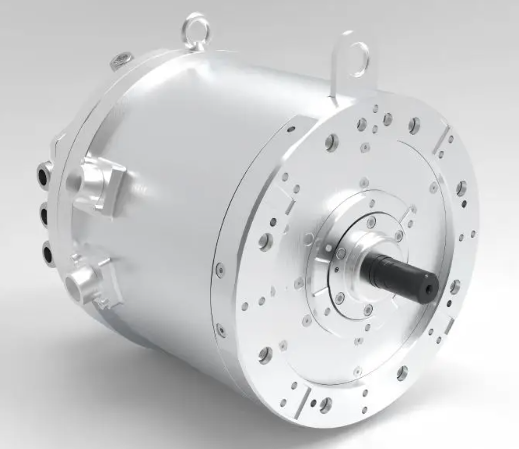
The motivation for this research comes from the operating profile of modern electric drives. A PMSM electric motor in a vehicle must repeatedly accelerate, climb, cruise, regenerate, and respond to sudden load changes. During these processes, the stator current may vary over a wide range, and the iron core may enter partial or deep saturation. The d-axis and q-axis magnetic paths interact, so a change in q-axis current can alter the d-axis inductance, and a change in d-axis current can alter the q-axis inductance. If the torque estimator ignores this behavior, the PMSM electric motor model will contain a persistent parameter mismatch. The consequences include biased torque feedback, poor torque sharing, unnecessary current ripple, and degraded efficiency. My goal is to treat the time-varying inductance not as an external disturbance to be rejected, but as an internal state-related parameter to be identified and embedded online.
1. Review of Control and Estimation Background
Field-oriented control, direct torque control, and model predictive control are widely used for the PMSM electric motor. Among them, field-oriented control with space vector pulse width modulation is still the most common industrial solution because it provides decoupled current control and stable steady-state behavior. In field-oriented control, the stator current is transformed into a d-q rotating frame aligned with the rotor flux. The torque of the PMSM electric motor is then controlled through the q-axis current and, in the case of an interior PMSM electric motor, also through the d-axis current. Maximum torque per ampere control is often used because it minimizes copper loss for a given torque demand. However, maximum torque per ampere control relies on accurate inductance values. If $L_d$ and $L_q$ are wrong, the current reference generated by maximum torque per ampere control is also wrong, and the torque estimation error increases.
Direct torque control has the advantage of fast torque response, but it suffers from torque and flux ripple because of hysteresis comparators. Model predictive control can handle multiple objectives and constraints, but its performance depends heavily on model accuracy. For all these strategies, the PMSM electric motor model is the foundation. The more accurately the inductances are known, the more reliable the torque estimate becomes. This is especially true for interior PMSM electric motor drives, where the saliency difference between $L_d$ and $L_q$ contributes to reluctance torque. A fixed-inductance model cannot capture the saturation-induced saliency variation, so the estimated torque may be significantly biased even when the current control loop appears stable.
2. Mathematical Model of the PMSM Electric Motor
I begin with the three-phase natural coordinate model of the PMSM electric motor. The stator voltage equations in the abc frame are expressed as
$$
\begin{aligned}
u_a &= R_s i_a + \frac{d\psi_a}{dt}, \\
u_b &= R_s i_b + \frac{d\psi_b}{dt}, \\
u_c &= R_s i_c + \frac{d\psi_c}{dt}.
\end{aligned}
$$
Here, $u_a$, $u_b$, and $u_c$ are the phase voltages, $i_a$, $i_b$, and $i_c$ are the phase currents, $R_s$ is the stator resistance, and $\psi_a$, $\psi_b$, and $\psi_c$ are the phase flux linkages. The flux linkages are related to the currents and the permanent magnet flux through the inductance matrix. Because the inductances vary with rotor position and magnetic saturation, the abc-frame model is accurate but inconvenient for real-time control. Coordinate transformation is therefore used to simplify the model of the PMSM electric motor.
The Clarke transformation converts the abc quantities into the stationary $\alpha\beta$ frame. With the amplitude-invariant form, the transformation matrix is
$$
T_{3s/2s} = \frac{2}{3}
\begin{bmatrix}
1 & -\frac{1}{2} & -\frac{1}{2} \\
0 & \frac{\sqrt{3}}{2} & -\frac{\sqrt{3}}{2}
\end{bmatrix}.
$$
The Park transformation then converts the stationary frame into the rotating d-q frame aligned with the rotor flux of the PMSM electric motor:
$$
T_{2s/2r} =
\begin{bmatrix}
\cos\theta_e & \sin\theta_e \\
-\sin\theta_e & \cos\theta_e
\end{bmatrix}.
$$
After these transformations, the voltage equations in the d-q frame are
$$
\begin{aligned}
u_d &= R_s i_d + \frac{d\psi_d}{dt} – \omega_e \psi_q, \\
u_q &= R_s i_q + \frac{d\psi_q}{dt} + \omega_e \psi_d,
\end{aligned}
$$
where $\omega_e$ is the electrical angular speed. The flux linkages are
$$
\begin{aligned}
\psi_d &= L_d i_d + \psi_f, \\
\psi_q &= L_q i_q,
\end{aligned}
$$
and the electromagnetic torque of the PMSM electric motor is
$$
T_e = \frac{3}{2} n_p \left[ \psi_f i_q + (L_d – L_q) i_d i_q \right],
$$
where $n_p$ is the number of pole pairs and $\psi_f$ is the permanent magnet flux linkage. This torque expression shows that the PMSM electric motor produces both permanent magnet torque and reluctance torque. The reluctance torque depends directly on the difference between $L_d$ and $L_q$. If saturation reduces this difference, the torque production capability changes. Therefore, a torque estimator that assumes constant $L_d$ and $L_q$ cannot remain accurate over the full operating range.
In the stationary $\alpha\beta$ frame, the voltage equation can be written as
$$
\begin{aligned}
u_\alpha &= R_s i_\alpha + L_\alpha \frac{di_\alpha}{dt} + L_{\alpha\beta} \frac{di_\beta}{dt} + e_\alpha, \\
u_\beta &= R_s i_\beta + L_{\beta\alpha} \frac{di_\alpha}{dt} + L_\beta \frac{di_\beta}{dt} + e_\beta,
\end{aligned}
$$
where the inductances are position-dependent:
$$
\begin{aligned}
L_\alpha &= L_0 + L_1 \cos(2\theta_e), \\
L_\beta &= L_0 – L_1 \cos(2\theta_e), \\
L_{\alpha\beta} &= L_1 \sin(2\theta_e),
\end{aligned}
$$
with
$$
L_0 = \frac{L_d + L_q}{2}, \qquad L_1 = \frac{L_d – L_q}{2}.
$$
These expressions reveal that the PMSM electric motor has a position-dependent inductance matrix in the stationary frame. This is one reason why direct flux integration from the stationary voltage model is sensitive to parameter errors. The extended flux concept used later in this work avoids some of these difficulties by rearranging the model into a symmetric form.
3. Space Vector Pulse Width Modulation and Maximum Torque per Ampere Control
For the PMSM electric motor drive, I use space vector pulse width modulation to synthesize the reference voltage. A two-level voltage source inverter has eight switching states: six active vectors and two zero vectors. The active vectors divide the complex plane into six sectors. In each switching period, the reference voltage vector is approximated by two adjacent active vectors and a zero vector. The volt-second balance is
$$
T_s \mathbf{u}_{out} = T_1 \mathbf{u}_1 + T_2 \mathbf{u}_2 + T_0 \mathbf{u}_0,
$$
where $T_s$ is the switching period, $T_1$ and $T_2$ are the active vector times, and $T_0$ is the zero vector time. The times are calculated from the sector and the reference voltage components. Space vector pulse width modulation provides a higher DC-link utilization than sinusoidal pulse width modulation and produces lower current harmonics. This benefits the PMSM electric motor because lower current harmonics reduce torque ripple and improve the accuracy of current-based estimation.
For torque control, I adopt maximum torque per ampere. The current vector angle is selected so that the PMSM electric motor produces the required torque with minimum stator current magnitude. The d-axis and q-axis currents satisfy
$$
i_d = -i_s \sin\beta, \qquad i_q = i_s \cos\beta,
$$
where $\beta$ is the current angle relative to the q-axis. Substituting into the torque equation gives
$$
T_e = \frac{3}{2} n_p \left[ \psi_f i_s \cos\beta – (L_d – L_q) i_s^2 \sin\beta \cos\beta \right].
$$
Differentiating with respect to $\beta$ and setting the derivative to zero leads to the maximum torque per ampere condition. The resulting current references depend on $L_d$ and $L_q$. When these inductances vary, the maximum torque per ampere trajectory shifts. Thus, online inductance identification is necessary not only for torque estimation but also for accurate current reference generation in the PMSM electric motor controller.
4. Torque Estimation Error Caused by Fixed Inductance
I now quantify the torque estimation error caused by using fixed inductances. Let the nominal fixed inductances be $L_{d0}$ and $L_{q0}$. The estimated torque of the PMSM electric motor is
$$
\hat{T}_e = \frac{3}{2} n_p \left[ \psi_f i_q + (L_{d0} – L_{q0}) i_d i_q \right].
$$
The true torque is
$$
T_e = \frac{3}{2} n_p \left[ \psi_f i_q + (L_d – L_q) i_d i_q \right].
$$
The absolute torque estimation error is therefore
$$
\Delta T_e = T_e – \hat{T}_e = \frac{3}{2} n_p i_d i_q \left[ (L_d – L_{d0}) – (L_q – L_{q0}) \right].
$$
Define the parameter deviations as
$$
\Delta L_d = L_d – L_{d0}, \qquad \Delta L_q = L_q – L_{q0}.
$$
Then
$$
\Delta T_e = \frac{3}{2} n_p i_d i_q (\Delta L_d – \Delta L_q).
$$
This compact expression shows that the torque estimation error of the PMSM electric motor is proportional to the product of the d-axis and q-axis currents and to the difference between the inductance deviations. In an interior PMSM electric motor under maximum torque per ampere control, $i_d$ is negative and $i_q$ is positive. Therefore, the sign and magnitude of the error depend on saturation and cross-coupling.
The relative torque estimation error is defined as
$$
\delta_{T_e} = \frac{|\Delta T_e|}{|T_e|} \times 100\%.
$$
I present the influence of single-parameter and coupled-parameter variations in Table 1. The table summarizes how a positive or negative inductance deviation affects the estimated torque under typical maximum torque per ampere operation.
| Condition | Inductance deviation | Current relation | Effect on estimated torque |
|---|---|---|---|
| d-axis inductance only | $\Delta L_d > 0$ | $i_d 0$ | Estimated torque becomes larger |
| d-axis inductance only | $\Delta L_d 0$ | $i_d 0$ | Estimated torque becomes smaller |
| q-axis inductance only | $\Delta L_q 0$ | $i_d 0$ | Estimated torque becomes larger |
| q-axis inductance only | $\Delta L_q > 0$ | $i_d 0$ | Estimated torque becomes smaller |
| coupled saturation at heavy load | $\Delta L_q 0$, $\Delta L_d 0$, $|\Delta L_q|>|\Delta L_d|$ | $i_d 0$ | Estimated torque becomes larger |
| deep field weakening | $\Delta L_d > 0$, $\Delta L_q > 0$, $\Delta L_d > \Delta L_q$ | $i_d 0$ | Estimated torque becomes larger |
Table 1 shows that the sign of the error is not fixed. It depends on the operating point. In low-speed light-load conditions, the inductances are close to their nominal values, so the error is small. In heavy-load conditions, q-axis saturation reduces $L_q$ strongly, and cross-coupling reduces $L_d$ as well. In high-speed field-weakening conditions, the negative d-axis current can increase $L_d$ and slightly increase $L_q$, but the difference between the deviations still produces a torque estimation error. This analysis confirms that online inductance identification is essential for a high-performance PMSM electric motor drive.
5. Online Inductance Identification Using Variable-Step ADALINE
To identify $L_d$ and $L_q$ online, I use an adaptive linear neuron, abbreviated as ADALINE. The ADALINE is a single-layer linear neural network that updates its weights by the least mean square rule. It is simple enough for embedded implementation and can track time-varying parameters when the step size is properly designed. The basic structure contains an input vector, a weight vector, a linear output, and an error signal. The weight update law is
$$
W(k+1) = W(k) + \eta(k) U(k) \varepsilon(k),
$$
where $W(k)$ is the weight vector, $U(k)$ is the input vector, $\varepsilon(k)$ is the estimation error, and $\eta(k)$ is the step size. For the PMSM electric motor, the weights correspond to the inductances to be identified.
I reconstruct the d-q voltage equations into a linear parameterized form. The voltage equations are
$$
\begin{aligned}
u_d &= R_s i_d + L_d \frac{di_d}{dt} – \omega_e L_q i_q, \\
u_q &= R_s i_q + L_q \frac{di_q}{dt} + \omega_e L_d i_d + \omega_e \psi_f.
\end{aligned}
$$
Rearranging gives
$$
\begin{bmatrix}
u_d – R_s i_d \\
u_q – R_s i_q – \omega_e \psi_f
\end{bmatrix}
=
\begin{bmatrix}
\frac{di_d}{dt} & -\omega_e i_q \\
\omega_e i_d & \frac{di_q}{dt}
\end{bmatrix}
\begin{bmatrix}
L_d \\
L_q
\end{bmatrix}.
$$
This is a linear regression model with unknown parameters $L_d$ and $L_q$. For real-time implementation, the derivatives are approximated by backward differences or filtered differences. The input vector and the desired output vector are constructed from measured voltages, currents, and electrical speed. The weight vector is
$$
W(k) =
\begin{bmatrix}
L_d(k) \\
L_q(k)
\end{bmatrix}.
$$
The error vector drives the adaptation. To balance fast tracking and steady-state accuracy, I use a variable step size that depends on the squared error:
$$
\eta(k) = \beta \left( 1 – \frac{1}{1 + \alpha |\varepsilon(k)|^2} \right),
$$
where $\alpha > 0$ is a shape factor and $\beta > 0$ is the maximum step size. When the error is large, the step size approaches $\beta$, which provides fast convergence. When the error is small, the step size decreases automatically, which suppresses noise and reduces steady-state oscillation. This is particularly important for the PMSM electric motor because the voltage and current measurements contain switching ripple and quantization noise. A fixed step size would force a tradeoff between convergence speed and steady-state accuracy. The variable step size avoids this tradeoff.
The convergence condition for the least mean square algorithm requires
$$
0 < \eta(k) < \frac{2}{\|U(k)\|^2}.
$$
I enforce this condition numerically by limiting the step size. The identified inductances are then embedded into the observer model. This creates a parameter-adaptive structure for the PMSM electric motor. The inductance identification is not an isolated block; it feeds the extended flux observer and the torque estimator in real time.
6. Simulation Study of Inductance Identification
I built a simulation platform for the PMSM electric motor in MATLAB/Simulink. The machine model includes saturation and cross-coupling through two-dimensional lookup tables for $L_d$ and $L_q$ as functions of speed and torque. The main parameters are listed in Table 2.
| Parameter | Value |
|---|---|
| DC bus voltage | 610 V |
| Stator resistance | 0.02 $\Omega$ |
| Permanent magnet flux linkage | 0.1 Wb |
| Rated speed | 1800 r/min |
| Rated torque | 80 N·m |
| Number of pole pairs | 4 |
| Nominal d-axis inductance | 9.8 mH |
| Nominal q-axis inductance | 21.9 mH |
I tested three representative conditions. The first is a high-speed ramp load at 1800 r/min. The second is a high-speed step load at 1800 r/min. The third is a low-speed step load at 300 r/min. In each case, I compare the proposed variable-step ADALINE method with an ordinary least squares method. The ordinary least squares method is used as a baseline because it is simple and widely known, but it is sensitive to noise and parameter drift.
In the 1800 r/min ramp load condition, the PMSM electric motor starts from zero speed, accelerates to rated speed, runs at no load, and then receives a load that rises uniformly to 70 N·m. The true d-axis inductance decreases from about 9.8 mH to about 7.5 mH because of saturation. The proposed method tracks this decrease with a steady-state error within $\pm 1.8\%$. The ordinary least squares method shows an error within $\pm 3.5\%$. The q-axis inductance decreases from about 21.9 mH to about 18.8 mH, and the proposed method keeps the error within $\pm 1.9\%$, while the ordinary least squares method reaches about $\pm 4\%$. These results are summarized in Table 3.
| Condition | Inductance | True final value | Proposed method error | OLS method error |
|---|---|---|---|---|
| 1800 r/min ramp load | $L_d$ | 7.5 mH | $\pm 1.8\%$ | $\pm 3.5\%$ |
| 1800 r/min ramp load | $L_q$ | 18.8 mH | $\pm 1.9\%$ | $\pm 4.0\%$ |
| 1800 r/min step load | $L_d$ | 6.3 mH | $\pm 1.9\%$ | $\pm 5.0\%$ |
| 1800 r/min step load | $L_q$ | 18.6 mH | $\pm 2.0\%$ | $\pm 4.8\%$ |
| 300 r/min step load | $L_d$ | 9.6 mH | $\pm 1.9\%$ | $\pm 3.5\%$ |
| 300 r/min step load | $L_q$ | 21.5 mH | $\pm 1.9\%$ | $\pm 2.9\%$ |
In the 1800 r/min step load condition, the load changes suddenly from 0 N·m to 80 N·m. The inductance change is also sudden. The proposed method shows a small overshoot and then converges quickly. The ordinary least squares method shows a larger overshoot and a slower recovery. This confirms that the variable step size improves the transient response of the PMSM electric motor parameter identification. In the 300 r/min step load condition, the load changes from 0 N·m to 30 N·m. The inductance variation is smaller, but the low-speed condition makes voltage measurement errors more significant. The proposed method still maintains an error within $\pm 2\%$, which is better than the ordinary least squares method.
7. Extended Flux Observer for Torque Estimation
After identifying the inductances, I use them in an extended flux observer. The extended flux is a transformed quantity that combines the permanent magnet flux and the saliency-induced flux. In the stationary $\alpha\beta$ frame, the extended flux is defined as
$$
\begin{bmatrix}
\psi_{1\alpha} \\
\psi_{1\beta}
\end{bmatrix}
=
\begin{bmatrix}
(L_d – L_q) i_d + \psi_f
\end{bmatrix}
\begin{bmatrix}
\cos\theta_e \\
\sin\theta_e
\end{bmatrix}.
$$
The stator flux linkage is related to the extended flux by
$$
\begin{bmatrix}
\psi_\alpha \\
\psi_\beta
\end{bmatrix}
=
\begin{bmatrix}
\psi_{1\alpha} \\
\psi_{1\beta}
\end{bmatrix}
+
L_q
\begin{bmatrix}
i_\alpha \\
i_\beta
\end{bmatrix}.
$$
The voltage equation in the stationary frame can then be written in a symmetric form:
$$
\begin{bmatrix}
u_\alpha \\
u_\beta
\end{bmatrix}
=
\begin{bmatrix}
R_s + D L_q & 0 \\
0 & R_s + D L_q
\end{bmatrix}
\begin{bmatrix}
i_\alpha \\
i_\beta
\end{bmatrix}
+
D
\begin{bmatrix}
\psi_{1\alpha} \\
\psi_{1\beta}
\end{bmatrix}.
$$
This form is convenient for observer design because the inductance matrix is diagonal. The extended flux dynamics satisfy
$$
D
\begin{bmatrix}
\psi_{1\alpha} \\
\psi_{1\beta}
\end{bmatrix}
=
\omega_e
\begin{bmatrix}
0 & -1 \\
1 & 0
\end{bmatrix}
\begin{bmatrix}
\psi_{1\alpha} \\
\psi_{1\beta}
\end{bmatrix}.
$$
I define the matrix
$$
J =
\begin{bmatrix}
0 & -1 \\
1 & 0
\end{bmatrix}.
$$
Then the extended flux state equation is
$$
D \psi_{1\alpha\beta} = \omega_e J \psi_{1\alpha\beta}.
$$
The output equation is obtained from the voltage equation:
$$
y = u_{\alpha\beta} – R_s i_{\alpha\beta} – L_q D i_{\alpha\beta} = \omega_e J \psi_{1\alpha\beta}.
$$
The electromagnetic torque can also be expressed through the extended flux:
$$
T_e = \frac{3}{2} n_p \left( \psi_{1\alpha} i_\beta – \psi_{1\beta} i_\alpha \right).
$$
This expression is useful because it does not require the rotor position explicitly once the extended flux is observed. The extended flux observer therefore provides a robust torque estimation structure for the PMSM electric motor.
8. Minimal-Order State Observer and Pole Placement
I design a minimal-order state observer for the extended flux. The general state observer has the form
$$
\dot{\hat{x}} = A \hat{x} + B u + K (y – \hat{y}),
$$
where $K$ is the observer gain matrix. For the extended flux model, the system matrices are
$$
A = \omega_e J, \qquad C = \omega_e J.
$$
The observer error dynamics are governed by
$$
\dot{\tilde{x}} = (A – K C) \tilde{x}.
$$
To eliminate the coupling between the $\alpha$ and $\beta$ axes, I choose the gain matrix in the form
$$
K =
\begin{bmatrix}
1 & -k \\
k & 1
\end{bmatrix}.
$$
Substituting this into the error dynamics gives
$$
\dot{\tilde{\psi}}_{1\alpha\beta} = -k \omega_e \tilde{\psi}_{1\alpha\beta}.
$$
The solution is
$$
\tilde{\psi}_{1\alpha\beta}(t) = \tilde{\psi}_{1\alpha\beta}(0) e^{-k \omega_e t}.
$$
This shows that the observation error decays exponentially when $k \omega_e > 0$. The parameter $k$ therefore controls the convergence speed and damping of the observer. If $k$ is too small, the observer responds slowly. If $k$ is too large, the observer amplifies measurement noise. Because the PMSM electric motor operates over a wide speed range, a fixed $k$ is not optimal. I therefore design a two-dimensional lookup table for $k$ as a function of speed and torque.
The gain design follows three principles. At low speed, the back electromotive force is small, so $k$ should be relatively large to compensate for the weak signal. At high speed, the back electromotive force is large, but the switching noise and current ripple are also more significant, so $k$ should be reduced to prevent noise amplification. Under heavy load, the parameter variation and cross-coupling are stronger, so $k$ should be increased to improve robustness. These principles are summarized in Table 4.
| Region | Speed range | Torque range | Weighting strategy | Typical $k$ range |
|---|---|---|---|---|
| I | 0–300 r/min | 0–20 N·m | Favor convergence and noise rejection | 1.8–3.5 |
| II | 0–300 r/min | 20–80 N·m | Favor robustness under heavy load | 2.2–4.0 |
| III | 300–900 r/min | 0–30 N·m | Balance convergence and noise | 1.0–2.7 |
| IV | 300–900 r/min | 30–80 N·m | Increase damping under load | 1.4–3.2 |
| V | 900–1800 r/min | 0–40 N·m | Reduce noise sensitivity | 0.6–1.8 |
| VI | 900–1800 r/min | 40–80 N·m | Balance high-speed noise and load robustness | 0.9–2.4 |
With this gain scheduling, the extended flux observer remains stable and accurate across the full operating range of the PMSM electric motor. The identified inductances from the variable-step ADALINE are updated online and used in the observer. This creates the closed-loop chain: online inductance identification, extended flux observation, and torque estimation.
9. Simulation Results of Torque Estimation
I embedded the proposed inductance identification, the ordinary least squares identification, and fixed nominal inductances into the same extended flux observer. I then compared the estimated torque with the actual torque under the three representative conditions. The results are summarized in Table 5.
| Condition | Proposed method steady-state error | OLS identification method steady-state error | Fixed inductance method steady-state error |
|---|---|---|---|
| 1800 r/min ramp load | $\pm 1.8\%$ | $\pm 4.0\%$ | $\pm 6.0\%$ |
| 1800 r/min step load | $\pm 2.0\%$ | $\pm 5.0\%$ | $\pm 8.0\%$ |
| 300 r/min step load | $\pm 1.9\%$ | $\pm 4.0\%$ | $\pm 5.0\%$ |
The simulation results show that the proposed method consistently provides the lowest torque estimation error. The fixed inductance method has the largest error because it does not compensate for saturation or cross-coupling. The ordinary least squares method improves the accuracy compared with the fixed inductance method, but its tracking ability is limited, especially during sudden load changes. The proposed method combines fast tracking with low steady-state error. This is important for the PMSM electric motor because torque estimation is used for torque control, efficiency optimization, and fault detection.
10. Experimental Platform and Validation
I validated the proposed method on an experimental platform for the PMSM electric motor. The control algorithms were generated from MATLAB/Simulink code generation and deployed on an NXP S32K144 microcontroller. The platform includes a power drive module, current and voltage sampling circuits, an encoder interface, and a high-precision torque sensor. The real d-axis and q-axis inductances were obtained by offline calibration and used as reference values for evaluating the online identification accuracy.
The experimental conditions match the simulation conditions. First, the PMSM electric motor runs at 1800 r/min and receives a ramp load rising to 70 N·m. Second, it runs at 1800 r/min and receives a step load of 80 N·m. Third, it runs at 300 r/min and receives a step load of 30 N·m. In each test, I compare the proposed method with the ordinary least squares identification method and the fixed inductance method.
In the high-speed ramp load test, the speed rises to 1800 r/min with about 5% overshoot and then stabilizes. When the load is applied, the speed drops by about 3% and recovers within about 0.3 s. The d-axis inductance decreases from about 9.8 mH to about 6.6 mH, and the q-axis inductance decreases from about 21.9 mH to about 16.4 mH. The proposed identification method tracks these changes with a steady-state error within $\pm 2.8\%$. The ordinary least squares method shows an error within $\pm 5\%$. For torque estimation, the proposed method keeps the steady-state error within $\pm 2.5\%$, while the ordinary least squares method reaches about $\pm 5\%$ and the fixed inductance method reaches about $\pm 7.5\%$. These results are listed in Table 6.
| Condition | Method | $L_d$ identification error | $L_q$ identification error | Torque estimation error |
|---|---|---|---|---|
| 1800 r/min ramp load | Proposed | $\pm 2.8\%$ | $\pm 2.8\%$ | $\pm 2.5\%$ |
| 1800 r/min ramp load | OLS | $\pm 5.0\%$ | $\pm 5.0\%$ | $\pm 5.0\%$ |
| 1800 r/min ramp load | Fixed inductance | Not applicable | Not applicable | $\pm 7.5\%$ |
In the high-speed step load test, the speed rises to 1800 r/min with about 5% overshoot. When an 80 N·m load is applied, the speed drops by about 8% and recovers within about 0.8 s. The d-axis inductance drops to about 6.3 mH, and the q-axis inductance drops to about 15.9 mH. The proposed method shows an overshoot of about 7.2 mH in the d-axis inductance and about 8.5 mH in the q-axis inductance. The ordinary least squares method shows larger overshoots of about 8.3 mH and 9.5 mH. The steady-state identification error of the proposed method is within $\pm 2.7\%$ for $L_d$ and $\pm 2.9\%$ for $L_q$. The ordinary least squares method reaches $\pm 6.6\%$ and $\pm 6.4\%$. The torque estimation error of the proposed method is within $\pm 2.8\%$, while the ordinary least squares method reaches $\pm 7.5\%$ and the fixed inductance method reaches $\pm 10\%$. Table 7 summarizes the comparison.
| Method | $L_d$ steady-state error | $L_q$ steady-state error | $L_d$ overshoot | $L_q$ overshoot | Torque estimation error |
|---|---|---|---|---|---|
| Proposed | $\pm 2.7\%$ | $\pm 2.9\%$ | 7.2 mH | 8.5 mH | $\pm 2.8\%$ |
| OLS | $\pm 6.6\%$ | $\pm 6.4\%$ | 8.3 mH | 9.5 mH | $\pm 7.5\%$ |
| Fixed inductance | Not applicable | Not applicable | Not applicable | Not applicable | $\pm 10.0\%$ |
In the low-speed step load test, the PMSM electric motor runs at 300 r/min. The speed rises with about 3% overshoot and recovers after the load is applied. The d-axis inductance remains around 9.6 mH, and the q-axis inductance remains around 21.2 mH. The proposed method shows an overshoot of about 0.8 mH in $L_d$ and about 1.1 mH in $L_q$. The ordinary least squares method shows overshoots of about 1.1 mH and 1.3 mH. The steady-state identification error of the proposed method is within $\pm 2.6\%$ for $L_d$ and $\pm 3.0\%$ for $L_q$. The ordinary least squares method reaches $\pm 4.0\%$ and $\pm 3.9\%$. The torque estimation error of the proposed method is within $\pm 2.6\%$, while the ordinary least squares method reaches $\pm 4\%$ and the fixed inductance method reaches $\pm 6\%$. These results are listed in Table 8.
| Method | $L_d$ steady-state error | $L_q$ steady-state error | $L_d$ overshoot | $L_q$ overshoot | Torque estimation error |
|---|---|---|---|---|---|
| Proposed | $\pm 2.6\%$ | $\pm 3.0\%$ | 0.8 mH | 1.1 mH | $\pm 2.6\%$ |
| OLS | $\pm 4.0\%$ | $\pm 3.9\%$ | 1.1 mH | 1.3 mH | $\pm 4.0\%$ |
| Fixed inductance | Not applicable | Not applicable | Not applicable | Not applicable | $\pm 6.0\%$ |
The experimental results confirm the simulation findings. The proposed variable-step ADALINE method identifies the dynamic inductances of the PMSM electric motor with high accuracy. When the identified inductances are embedded into the extended flux observer, the torque estimation error remains within $\pm 2.8\%$ under all tested conditions. The ordinary least squares method and the fixed inductance method show larger errors, especially during sudden load changes. This validates the effectiveness of the closed-loop scheme for the PMSM electric motor.
11. Discussion of Advantages and Limitations
The main advantage of the proposed method is that it treats inductance variation as a real-time parameter rather than a fixed constant. This reduces model mismatch in the PMSM electric motor. The variable-step ADALINE provides a good balance between convergence speed and steady-state noise suppression. The extended flux observer provides a symmetric and stable structure for flux observation. The gain scheduling of $k$ adapts the observer to different speed and torque regions. The combination of these techniques improves torque estimation accuracy without requiring additional hardware beyond the standard voltage, current, and position sensors.
There are also limitations. The method relies on voltage and current measurements. In very low-speed conditions, the voltage signal is small, and measurement noise can degrade identification accuracy. In deep field-weakening conditions, the inductance variation is complex, and the linearized voltage model may not capture all saturation effects. The computational burden is moderate but not negligible for low-cost microcontrollers. Further optimization of the algorithm structure and fixed-point implementation may be needed for mass production. Temperature variation also affects stator resistance and permanent magnet flux, which are assumed constant in this work. Future research can include temperature adaptation and more advanced disturbance rejection.
12. Conclusion and Future Work
In this work, I developed a dynamic inductance-aware torque estimation method for the PMSM electric motor. I established multi-coordinate mathematical models, derived the torque estimation error caused by fixed inductance, and designed an online inductance identification algorithm based on variable-step ADALINE. I then constructed a parameter-adaptive extended flux observer with pole placement and two-dimensional gain scheduling. The identified inductances were embedded into the observer to form a closed-loop torque estimation scheme. Simulation and experimental results under high-speed ramp load, high-speed step load, and low-speed step load conditions showed that the proposed method keeps the steady-state torque estimation error within $\pm 2.8\%$, which is significantly better than the ordinary least squares identification method and the fixed inductance method. The proposed scheme effectively compensates for magnetic saturation and cross-coupling in the PMSM electric motor.
For future work, I plan to enhance the observer with sliding-mode or extended state observation techniques to improve disturbance rejection. I will test the method under extreme field weakening, high temperature, and severe measurement noise. I will also investigate event-triggered or reduced-order implementations to lower the computational cost. These extensions can make the dynamic inductance-aware torque estimation method more suitable for next-generation PMSM electric motor drives in electric vehicles and industrial automation.