
High-end precision equipment — computer numerical control machine tools, semiconductor lithography stages, wafer handling robots, and precision assembly platforms — derives its achievable machining accuracy and throughput almost entirely from the quality of the underlying servo drive. Among all candidate actuators, the permanent magnet synchronous motor has become the default choice for such applications because of its high power density, high efficiency, high torque-to-inertia ratio, and excellent speed-regulation characteristics. Despite these favorable electromagnetic properties, a permanent magnet synchronous motor operating inside a real position servo loop is continuously subjected to a superposition of heterogeneous disturbances: parameter drift caused by thermal variation of stator resistance and permanent magnet flux linkage, nonlinear friction in the guideways and bearings, cogging torque harmonics produced by the interaction between the stator slots and the rotor magnets, unmodeled high-frequency dynamics originating from mechanical resonance and transmission compliance, quantization noise in the encoder interface, and abrupt load torque changes imposed by the process itself. These effects jointly degrade tracking accuracy and disturb rejection capability, and they are precisely the reason why conventional control strategies struggle to satisfy modern performance specifications.
In this work I address the problem from two complementary directions at once. First, I replace the conventional single extended state observer with a cascaded active disturbance rejection control architecture, in which a second-order active disturbance rejection controller supervises the position loop and a first-order active disturbance rejection controller supervises the speed loop, so that low-frequency and mid-to-high-frequency disturbances are observed and compensated by structurally different observers with individually tunable bandwidths. Second, I recognize that the resulting controller exposes a comparatively large number of coupled nonlinear parameters whose manual tuning is both time-consuming and suboptimal, and I therefore deploy an improved differential evolution algorithm, equipped with Tent chaotic initialization and a Gaussian–Cauchy hybrid mutation mechanism, to search for the optimal parameter set automatically. The combination is referred to throughout this article as cascaded active disturbance rejection control driven by an improved differential evolution algorithm.
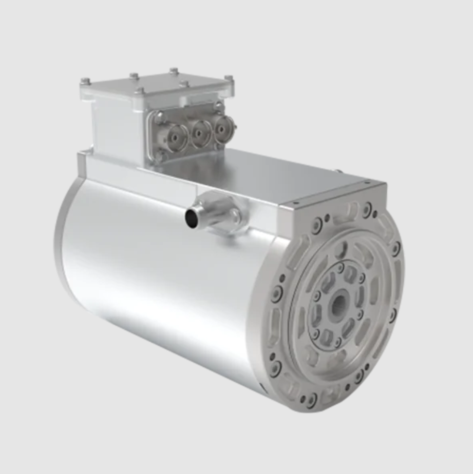
Mathematical Model of the Permanent Magnet Synchronous Motor
I begin from the three-phase stator voltage equations written in the natural ABC reference frame. For a permanent magnet synchronous motor with symmetrical windings and negligible magnetic saturation, the stator voltage balance reads
$$
\begin{bmatrix} u_A \\ u_B \\ u_C \end{bmatrix}
=
\begin{bmatrix} R_s & 0 & 0 \\ 0 & R_s & 0 \\ 0 & 0 & R_s \end{bmatrix}
\begin{bmatrix} i_A \\ i_B \\ i_C \end{bmatrix}
+
\frac{d}{dt}
\begin{bmatrix} \psi_A \\ \psi_B \\ \psi_C \end{bmatrix}
$$
where $u_A,u_B,u_C$ denote the three-phase stator voltages, $i_A,i_B,i_C$ the three-phase stator currents, $\psi_A,\psi_B,\psi_C$ the three-phase stator flux linkages, and $R_s$ the stator phase resistance. Because the inductances in the ABC frame are position dependent, this representation is unsuitable for controller synthesis. I therefore apply the Clarke transformation followed by the Park transformation and obtain the model in the $d$–$q$ synchronous rotating reference frame:
$$
\begin{bmatrix} u_d \\ u_q \end{bmatrix}
=
\begin{bmatrix} R_s & 0 \\ 0 & R_s \end{bmatrix}
\begin{bmatrix} i_d \\ i_q \end{bmatrix}
+
\begin{bmatrix} \dfrac{d}{dt} & -\omega_e \\[4pt] \omega_e & \dfrac{d}{dt} \end{bmatrix}
\begin{bmatrix} \psi_d \\ \psi_q \end{bmatrix}
$$
Here $u_d,u_q$ are the stator voltage components along the direct and quadrature axes, $i_d,i_q$ are the corresponding current components — the direct-axis current is also called the magnetizing current and the quadrature-axis current is also called the torque-producing current — $\psi_d,\psi_q$ are the flux linkage components, and $\omega_e$ is the electrical angular velocity of the rotor. The electromagnetic torque produced by the permanent magnet synchronous motor is
$$
T_e = \frac{3}{2} p_n \left[ \psi_f + (L_d – L_q)\, i_d \right] i_q
$$
where $p_n$ is the number of pole pairs, $\psi_f$ is the permanent magnet flux linkage, and $L_d, L_q$ are the direct- and quadrature-axis inductances. The mechanical dynamics obey
$$
J \frac{d\omega_m}{dt} = T_e – B\,\omega_m – T_L
$$
with $J$ the total moment of inertia referred to the motor shaft, $\omega_m$ the mechanical angular velocity related to the electrical angular velocity by $\omega_e = p_n \omega_m$, $B$ the viscous damping coefficient, and $T_L$ the load torque. For a surface-mounted permanent magnet synchronous motor the inductances are practically equal, $L_d \approx L_q$, so the reluctance torque term vanishes and the torque becomes proportional to the quadrature-axis current alone. Combining the torque equation with the mechanical equation yields a second-order description of the mechanical plant in which the measured position $\theta$ and the mechanical speed $\omega_m$ are the state variables:
$$
\ddot{\theta} = -\frac{B}{J}\omega_m + \frac{3 p_n \psi_f}{2 J} i_q – \frac{T_L}{J}
$$
Introducing the input gain $b_0 = \dfrac{3 p_n \psi_f}{2 J}$ and lumping the damping, the load torque, the unmodeled dynamics, and every other unknown disturbance into a single total disturbance signal $f$, the plant collapses to the canonical double-integrator form used by active disturbance rejection control:
$$
\ddot{\theta} = f + b_0 u , \qquad u = i_q
$$
This canonical form is the cornerstone of the entire design. It states that no matter how complicated the internal physics of the permanent magnet synchronous motor becomes, the input–output behavior seen by the position controller is a double integrator perturbed by an unknown, bounded, time-varying signal. The controller does not need an accurate model of $f$; it needs only a sufficiently fast and sufficiently accurate observer of $f$.
| Symbol | Quantity | Value | Unit |
|---|---|---|---|
| $p_n$ | Number of pole pairs | 5 | – |
| $R_s$ | Stator phase resistance | 1.45 | $\Omega$ |
| $L_d = L_q$ | Stator inductance | 4.2 | mH |
| $\psi_f$ | Permanent magnet flux linkage | 0.086 | Wb |
| $J$ | Total moment of inertia | $1.9 \times 10^{-4}$ | kg·m² |
| $B$ | Viscous damping coefficient | $3.2 \times 10^{-4}$ | N·m·s/rad |
| $T_{rated}$ | Rated torque | 1.27 | N·m |
| $n_{rated}$ | Rated speed | 3000 | r/min |
| $f_{PWM}$ | PWM carrier frequency | 16 | kHz |
| $f_s$ | Control sampling frequency | 8 | kHz |
| $N_{enc}$ | Encoder resolution | 10 000 | pulse/rev |
Conventional Active Disturbance Rejection Control
A conventional active disturbance rejection controller contains three functional blocks: a tracking differentiator, an extended state observer, and a nonlinear state-error feedback control law. The tracking differentiator serves a dual purpose. It arranges a smooth transient profile for the reference signal so that a step command does not immediately provoke overshoot, and it simultaneously extracts a usable derivative signal that the downstream control law can consume. For a reference $v$ the second-order tracking differentiator is
$$
\begin{cases}
\dot{v}_1 = v_2 \\[4pt]
\dot{v}_2 = \mathrm{fhan}(v_1 – v,\; v_2,\; r,\; h)
\end{cases}
$$
where $v_1$ tracks the reference, $v_2$ tracks the derivative of $v_1$, $r$ is the speed factor controlling how aggressively the differentiator follows the reference, and $h$ is the filtering factor governing noise suppression. The time-optimal control synthesis function $\mathrm{fhan}$ is defined by
$$
d = r h, \qquad d_0 = h\,d, \qquad y = x_1 + h\,x_2, \qquad a_0 = \sqrt{d^2 + 8 r |y|}
$$
$$
a =
\begin{cases}
x_2 + \dfrac{(a_0 – d)}{2}\,\mathrm{sign}(y), & |y| > d_0 \\[8pt]
x_2 + \dfrac{y}{h}, & |y| \le d_0
\end{cases}
$$
$$
\mathrm{fhan}(x_1,x_2,r,h) =
\begin{cases}
-r\,\mathrm{sign}(a), & |a| > d \\[8pt]
-r\,\dfrac{a}{d}, & |a| \le d
\end{cases}
$$
To estimate the total disturbance, I augment the state vector with the disturbance itself, setting $x_3 = f$ and assuming $\dot{x}_3 = h \approx 0$. The resulting third-order extended state space representation of the mechanical plant is
$$
\begin{cases}
\dot{x}_1 = x_2 \\
\dot{x}_2 = x_3 + b_0 u \\
\dot{x}_3 = h \approx 0 \\
y = x_1 = \theta
\end{cases}
$$
with $x_1 = \theta$ and $x_2 = \omega_m$. The corresponding nonlinear extended state observer is
$$
\begin{cases}
e = z_1 – y \\
\dot{z}_1 = z_2 – \beta_{01}\,\mathrm{fal}(e,\alpha_1,\delta) \\
\dot{z}_2 = z_3 + b_0 u – \beta_{02}\,\mathrm{fal}(e,\alpha_2,\delta) \\
\dot{z}_3 = -\beta_{03}\,\mathrm{fal}(e,\alpha_3,\delta)
\end{cases}
$$
in which $z_1,z_2,z_3$ are the observed versions of $x_1,x_2,x_3$, the observer gains $\beta_{01},\beta_{02},\beta_{03}$ are all strictly positive, and the nonlinear function $\mathrm{fal}$ is
$$
\mathrm{fal}(e,\alpha,\delta) =
\begin{cases}
\dfrac{e}{\delta^{1-\alpha}}, & |e| \le \delta \\[8pt]
|e|^{\alpha}\,\mathrm{sign}(e), & |e| > \delta
\end{cases}
$$
with $\alpha$ the nonlinear exponent and $\delta$ the width of the linear region. The state error between the tracking differentiator output and the observer output is formed as
$$
\begin{cases}
e_1 = v_1 – z_1 \\
e_2 = v_2 – z_2
\end{cases}
$$
and the nonlinear state error feedback law is
$$
u_0 = \beta_1\,\mathrm{fal}(e_1,\alpha_1,\delta) + \beta_2\,\mathrm{fal}(e_2,\alpha_2,\delta)
$$
Finally, the disturbance estimate is fed forward and cancelled at the control output:
$$
u = \frac{1}{b_0}\left(u_0 – \hat{f}\right), \qquad \hat{f} = z_3
$$
The practical difficulty with this construction, when it is applied to a permanent magnet synchronous motor position servo, is that a single observer must simultaneously estimate disturbances whose spectral content spans several decades. For an $n$-th order plant, the $(n+1)$-th order extended state observer exposes essentially one tuning knob, the observer bandwidth $\omega_o$, and that single bandwidth fixes both the speed with which the observer tracks a time-varying disturbance and the degree to which it amplifies measurement noise. Raising $\omega_o$ to catch fast load steps inevitably admits more encoder quantization noise and can trigger the well-known peaking phenomenon; lowering $\omega_o$ to protect the loop from noise inevitably introduces phase lag into the disturbance estimate, so that the compensation arrives late and the transient error grows. There is no single value of $\omega_o$ that is simultaneously optimal for slow thermal drift and for a fast load step.
| Observer bandwidth $\omega_o$ | Disturbance tracking speed | Noise amplification | Phase lag of $\hat{f}$ | Risk of peaking |
|---|---|---|---|---|
| Low | Slow | Very low | Large | Negligible |
| Moderate | Adequate for slow drift | Low | Moderate | Small |
| High | Fast | High | Small | Significant |
| Very high | Very fast | Very high | Negligible | Severe |
Cascaded Active Disturbance Rejection Control
My central architectural argument is that the disturbances acting on a permanent magnet synchronous motor position servo are not statistically homogeneous. They partition naturally into a low-frequency group and a mid-to-high-frequency group. The low-frequency group contains Coulomb and Stribeck friction, slow parameter drift caused by temperature rise in the stator winding and the magnets, and constant or slowly ramping load torque. The mid-to-high-frequency group contains step and square-wave load torque changes, cogging torque harmonics at the slot–pole interaction frequency, unmodeled high-frequency dynamics excited by mechanical resonance, and encoder quantization noise. Rather than forcing one observer to cover both bands, I assign each band to a dedicated observer embedded in a dedicated control loop.
The position-loop plant is written in the same canonical form as before,
$$
\ddot{\theta} = f_p(\theta,\dot{\theta},t) + b_p u_p
$$
where $f_p$ aggregates the speed-loop tracking error, external disturbances, and unmodeled dynamics referred to the position level, and the position loop is treated as a second-order system. I apply a second-order tracking differentiator, a third-order nonlinear extended state observer, and a nonlinear state error feedback law to this loop. The tracking differentiator is
$$
\begin{cases}
\dot{v}_{p1} = v_{p2} \\
\dot{v}_{p2} = \mathrm{fhan}(v_{p1} – \theta_{ref},\; v_{p2},\; r_p,\; h_p)
\end{cases}
$$
the position-loop observer is
$$
\begin{cases}
e_p = z_{p1} – \theta \\
\dot{z}_{p1} = z_{p2} – \beta_{p1}\,\mathrm{fal}(e_p,\alpha_{p1},\delta_p) \\
\dot{z}_{p2} = z_{p3} + b_p u_p – \beta_{p2}\,\mathrm{fal}(e_p,\alpha_{p2},\delta_p) \\
\dot{z}_{p3} = -\beta_{p3}\,\mathrm{fal}(e_p,\alpha_{p3},\delta_p)
\end{cases}
$$
and the position-loop control law is
$$
\begin{cases}
e_{p1} = v_{p1} – z_{p1} \\
e_{p2} = v_{p2} – z_{p2} \\
u_p = \dfrac{k_{pp}\,\mathrm{fal}(e_{p1},\alpha_{pp},\delta_{pp}) + k_{pd}\,\mathrm{fal}(e_{p2},\alpha_{pp},\delta_{pp}) – z_{p3}}{b_p}
\end{cases}
$$
The output $u_p = \omega_{ref}$ becomes the reference speed handed to the inner loop. The speed-loop plant of the permanent magnet synchronous motor is first order once the current loop is assumed to be sufficiently fast,
$$
\dot{\omega} = f_v(\omega,t) + b_v u_v
$$
where $f_v$ represents the equivalent disturbance arising from current-loop lag and mechanical parameter perturbation. Because this is a first-order plant, a first-order active disturbance rejection controller is the natural choice. Its tracking differentiator, observer, and control law are
$$
\dot{v}_1 = \mathrm{fhan}(v_1 – \omega_{ref},\, 0,\, r_v,\, h_v)
$$
$$
\begin{cases}
e_v = z_{v1} – \omega_{ref} \\
\dot{z}_{v1} = z_{v2} + b_v u_v – \beta_{v1}\,\mathrm{fal}(e_v,\alpha_{v2},\delta_v) \\
\dot{z}_{v2} = -\beta_{v2}\,\mathrm{fal}(e_v,\alpha_{v2},\delta_v)
\end{cases}
$$
$$
\begin{cases}
e_v = v_1 – z_{v1} \\
u_v = \dfrac{k_{vp}\,\mathrm{fal}(e_v,\alpha_{vp},\delta_{vp}) – z_{v2}}{b_v}
\end{cases}
$$
The output $u_v = i_q^{*}$ is the quadrature-axis current reference delivered to the current controller. Structurally, the position-loop observer handles the slow, large-amplitude, low-frequency components of the total disturbance, while the speed-loop observer handles the fast, smaller-amplitude, mid-to-high-frequency components. Because each observer is asked to cover a narrower band, each can be tuned with a bandwidth that is aggressive within its own band while remaining conservative outside it, and the classical trade-off summarized in Table 2 is substantially relaxed.
| Property | Conventional ADRC | Cascaded ADRC |
|---|---|---|
| Number of loops | One position loop with inner PI speed loop | Position loop plus speed loop, both ADRC |
| Observer order at position level | Third order | Third order |
| Observer order at speed level | None (PI controller) | Second order |
| Disturbance bands covered | Single band, fixed by $\omega_o$ | Two bands, each independently tunable |
| Load-step rejection | Limited by observer phase lag | Fast, handled by inner observer |
| Noise sensitivity | Compromise value | Outer observer kept slow, inner observer fast |
| Tuning burden | Moderate | Higher, motivates automated optimization |
| Model dependence | Low | Low |
The price of this improved disturbance handling is a larger parameter set. The observer gains $\beta_p$ and $\beta_v$, the control-law gains $k_p$ and $k_v$, and the compensation factors $b_p$ and $b_v$ dominate the closed-loop behavior, and they interact strongly. A change in the position observer bandwidth alters the effective reference seen by the speed loop, which in turn alters the disturbance profile that the speed observer must absorb. Manual trial-and-error tuning of such a coupled set is impractical in an industrial commissioning scenario, and heuristic sequential tuning rarely reaches the global optimum. This is the motivation for the optimization stage described next.
Improved Differential Evolution Algorithm
Differential evolution is a population-based global optimizer whose distinguishing feature is that it generates search directions from the difference vectors between randomly selected members of the current population. It requires no gradient information, it is conceptually simple, and it works well on the non-smooth, non-convex, multi-modal cost landscapes that typically arise when controller parameters are tuned against a time-domain performance index. The classical algorithm proceeds through initialization, mutation, crossover, and selection.
Within a search space $[X_{\min}, X_{\max}]$ a population $P = \{X_1, X_2, \dots, X_{NP}\}$ of size $NP$ is generated, and the $j$-th coordinate of the $i$-th individual is initialized as
$$
x_{i,j}(0) = x_{j,\min} + \mathrm{rand}(0,1)\cdot\left(x_{j,\max} – x_{j,\min}\right)
$$
where $\mathrm{rand}(0,1)$ is a uniformly distributed random number in the unit interval. Mutation then produces, for every target individual $X_i(g)$ at generation $g$, a mutant vector
$$
V_i(g) = x_{r1}(g) + F\cdot\left[x_{r2}(g) – x_{r3}(g)\right]
$$
where the indices $r_1, r_2, r_3 \in \{1,2,\dots,NP\}$ are drawn at random, are mutually distinct, and differ from the current target index $i$; the scaling factor $F>0$ controls the amplification of the differential perturbation. Binomial crossover then recombines the mutant vector with the target vector to form the trial vector $U_i(g) = [u_{i,1}(g), u_{i,2}(g), \dots, u_{i,D}(g)]$ coordinate by coordinate:
$$
u_{i,j}(g) =
\begin{cases}
v_{i,j}(g), & \mathrm{rand}_{i,j}(0,1) \le CR \ \text{or}\ j = j_{rand} \\[4pt]
x_{i,j}(g), & \text{otherwise}
\end{cases}
$$
Here $CR \in [0,1]$ is the crossover probability, and the condition $j = j_{rand}$ guarantees that at least one coordinate of the trial vector is inherited from the mutant, preventing the degenerate case in which the trial vector is an exact copy of the target. Selection is greedy:
$$
X_i(g+1) =
\begin{cases}
U_i(g), & f\!\left(U_i(g)\right) \le f\!\left(X_i(g)\right) \\[4pt]
X_i(g), & f\!\left(U_i(g)\right) > f\!\left(X_i(g)\right)
\end{cases}
$$
where $f(\cdot)$ is the fitness function. For a minimization problem, the trial vector replaces the target only when it is at least as good, so the population moves monotonically toward better regions of the search space.
Two well-documented weaknesses of this classical scheme matter for my application. Uniform random initialization can leave large regions of the search space unexplored, which wastes the expensive early generations. And a single mutation strategy based purely on differential vectors can stagnate once the population has contracted, because the differential perturbations become too small to escape a local basin. I therefore introduce two modifications.
Chaotic initialization using the Tent map
Chaotic maps combine ergodicity, boundedness, and sensitivity to initial conditions, and they produce initial populations that cover the search space far more uniformly than pseudo-random sampling. The logistic map is the most frequently cited choice, but its invariant density is markedly non-uniform, with a pronounced clustering of iterates near the extremes of the unit interval. The Tent map does not suffer from this defect. Its definition is
$$
x_{k+1} =
\begin{cases}
\dfrac{x_k}{a}, & 0 \le x_k < a \\[8pt]
\dfrac{1 – x_k}{1 – a}, & a \le x_k \le 1
\end{cases}
$$
where $x_k$ is the current chaotic variable, $x_{k+1}$ the next iterate, $x_0 \notin \{0, 0.25, 0.5, 0.75, 1\}$ to avoid fixed points, and $a$ is the control parameter. At $a = 0.5$ the Tent map exhibits a highly uniform invariant distribution. I set the population size to $NP = 500$ and generate the initial coordinates of each individual by mapping the chaotic sequence onto the corresponding parameter interval. The resulting uniformity translates directly into a lower probability of premature convergence and a faster reduction of the fitness value in the first few generations.
| Property | Logistic map | Tent map |
|---|---|---|
| Invariant density | Non-uniform, peaks near interval ends | Uniform for $a = 0.5$ |
| Coverage of search space | Moderate | High |
| Risk of clustered initial individuals | Elevated | Low |
| Sensitivity to initial value | High | High |
| Suitability for controller tuning | Acceptable | Preferred |
Gaussian–Cauchy hybrid mutation
To prevent the search from stagnating inside a local optimum, I augment the mutation operator with a hybrid random perturbation whose distribution switches between Gaussian and Cauchy according to a probability schedule. The revised mutation equation is
$$
V_i(g) = x_{r1}(g) + F\cdot\left[x_{r2}(g) – x_{r3}(g)\right] + \eta\cdot\Delta_{GC}
$$
where the hybrid perturbation term is
$$
\Delta_{GC} =
\begin{cases}
\mathcal{N}(0,\sigma^2), & \mathrm{rand}() < p_g \\[4pt]
\mathcal{C}(0,\gamma), & \mathrm{rand}() \ge p_g
\end{cases}
$$
and the perturbation strength decays with generation number according to
$$
\eta = \eta_{\max}\cdot\left(1 – \frac{g}{G_{\max}}\right)
$$
The rationale is that the Gaussian component concentrates its mass close to the mean and is therefore well suited to fine local exploitation, while the Cauchy component has heavy tails and can generate large jumps that carry an individual out of a local basin. By setting the mixing probability $p_g$ high early in the run so that Gaussian perturbations dominate, and low late in the run so that Cauchy perturbations dominate, the algorithm obtains strong early convergence followed by effective escape capability precisely when the population has contracted and stagnation would otherwise occur. Because $\eta$ decays toward zero, the perturbation vanishes as the run terminates, which preserves the final convergence accuracy that would otherwise be destroyed by persistent large-amplitude noise.
Encoding, fitness function, and observer gain parameterization
The observer gains of a nonlinear extended state observer are strongly correlated with its bandwidth. Rather than searching the three gains of each observer independently, which inflates the dimensionality of the problem and produces many equivalent solutions, I parameterize them through the bandwidth relations
$$
\beta_{01} = 2\omega_{c,ESO}, \qquad \beta_{02} = \omega_{c,ESO}^{2}, \qquad \beta_{03} = \omega_{c,ESO}^{3}
$$
This reduces each observer to a single bandwidth parameter that can be bounded from engineering considerations. The compensation factors $b_p$ and $b_v$ and the nonlinear exponents are pre-tuned from the nominal physical parameters listed in Table 1, since they are far less sensitive than the gains. I then use the improved differential evolution algorithm to optimize eight decision variables: the two observer bandwidths, the two sets of control-law gains, and the two speed-loop observer gains. The fitness function is the integral of time multiplied by the absolute error,
$$
\mathrm{IATE} = \int_{0}^{\infty} t\,\left|e(t)\right|\,dt
$$
where $e(t)$ is the difference between the reference and the measured position. The time weighting is deliberate. It penalizes errors that persist, not merely errors that are large, and therefore favors parameter sets that combine a fast initial rise with a small steady-state offset rather than sets that achieve a spectacularly fast rise at the cost of a long settling tail. A summary of the algorithmic configuration is given in Table 5.
| Element | Setting |
|---|---|
| Population size $NP$ | 500 |
| Maximum generations $G_{\max}$ | 100 |
| Scaling factor $F$ | 0.5 (fixed) |
| Crossover probability $CR$ | 0.9 |
| Initialization | Tent chaotic map, $a = 0.5$ |
| Mutation | Differential plus Gaussian–Cauchy hybrid |
| Perturbation strength | $\eta_{\max} = 0.15$, linearly decaying |
| Mixing schedule $p_g$ | $p_g = 0.8 \rightarrow 0.2$ over the run |
| Decision variables | 8 controller parameters |
| Fitness function | $\mathrm{IATE}$ |
| Constraint handling | Box bounds plus penalty on overshoot |
The complete workflow is as follows. I initialize $NP = 500$ individuals across the eight-dimensional search box using the Tent chaotic sequence. I evaluate each individual by simulating or executing the cascaded active disturbance rejection control loop on the permanent magnet synchronous motor platform and integrating the IATE cost. I apply the hybrid-mutation differential operator, perform binomial crossover, and apply greedy selection. The loop repeats for $G_{\max}$ generations, after which the best individual is extracted and written into the controller. Because the fitness evaluation involves a physical or simulated transient, I bound the search box conservatively to avoid parameter combinations that would destabilize the drive and endanger the hardware during the online search.
Experimental Evaluation
I built a test bench that comprises a programmable logic controller acting as the supervisory master, a linear joint module driven by a permanent magnet synchronous motor, and a commercial servo drive operating in torque-command mode with the current loop closed internally. A magnetic powder brake provides a controllable and abruptly switchable load torque. Position feedback comes from an incremental encoder mounted on the motor shaft. The nominal machine parameters are the ones listed in Table 1. All control algorithms run at 8 kHz on the drive’s digital signal processor, and the position reference is dispatched from the master over the fieldbus.
For a fair comparison I tuned both benchmark controllers, proportional–integral control and conventional single-observer active disturbance rejection control, by careful manual iteration until neither could be improved further on the same benchmark task. The cascaded active disturbance rejection controller was tuned exclusively by the improved differential evolution algorithm. Three scenarios were then executed: a large step position command to quantify tracking speed and steady-state accuracy, a small step position command to verify that the advantage persists at small signal amplitudes, and a 400 N step load torque applied at $t = 0.2$ s after the axis had settled to show disturbance rejection.
Step position tracking
In the large-step scenario the reference position is commanded to jump by a substantial fraction of the stroke. The time required to reach and remain within the steady-state band is recorded together with the residual steady-state error. The cascaded scheme outperformed both benchmarks by a wide margin. Relative to proportional–integral control and to conventional active disturbance rejection control, the step position response speed improved by 24.1 % to 70 %, and the steady-state position tracking error fell by 33.3 % to 71.4 %. The improvement is not a marginal refinement; it changes the servo from a device that visibly lags the command to one whose response is dominated by the commanded trajectory rather than by the controller’s own settling behavior.
| Metric | PI control | Conventional ADRC | Cascaded ADRC with improved DE |
|---|---|---|---|
| Rise time to 90 % (large step) | Baseline | Improved but slower than cascaded | Fastest |
| Response speed gain | Reference | +0 % to +24 % | +24.1 % to +70 % |
| Steady-state error (large step) | Baseline | Moderately reduced | Reduced by 33.3 % to 71.4 % |
| Overshoot | Present, tuning dependent | Small | Small, bounded by penalty term |
| Settling behavior | Long tail | Moderate | Short, monotone decay |
Two mechanisms explain the gain. The cascaded observer structure supplies a more accurate and less phase-lagged estimate of the total disturbance, so the feed-forward cancellation term removes a larger fraction of the perturbation before it can accumulate into position error. And the improved differential evolution optimizer finds a parameter combination in which the position-loop bandwidth, the speed-loop bandwidth, and the two nonlinear feedback laws are mutually consistent, which manual sequential tuning rarely achieves because the interactions are strongly non-separable.
Step load torque rejection
The disturbance rejection test is, in my assessment, the most informative of the three. After the axis settles at the commanded position, an abrupt step load torque of 400 N is applied at $t = 0.2$ s, and the resulting excursion of the measured position from its reference is recorded as the maximum position tracking error. Proportional–integral control produced an excursion of 60 pulses and needed approximately 0.6 s to return to the steady-state band. Conventional active disturbance rejection control produced an excursion of 86 pulses and needed approximately 0.8 s to recover. Cascaded active disturbance rejection control produced an excursion of only 3 pulses, and the position tracking error remained within an entirely acceptable band throughout the transient.
| Controller | Maximum position tracking error (pulse) | Recovery time (s) | Reduction relative to PI | Reduction relative to conventional ADRC |
|---|---|---|---|---|
| PI control | 60 | ≈ 0.6 | Reference | — |
| Conventional ADRC | 86 | ≈ 0.8 | — | Reference |
| Cascaded ADRC with improved DE | 3 | Negligible | 95.0 % | 96.5 % |
The fact that conventional active disturbance rejection control performs slightly worse than proportional–integral control in this specific test deserves comment, because it illustrates precisely the pathology that motivated the cascaded architecture. In the conventional scheme the single observer must be detuned to keep encoder noise out of the control signal, and the resulting phase lag means that the load step is detected only after the position error has already grown. When the compensation finally arrives it is both late and partially misestimated. Across the full set of load-step amplitudes tested, the cascaded method reduced the maximum position tracking error by 92.8 % to 96.5 % relative to the two benchmarks, and the axis recovered to the steady-state band quickly in every case.
| Performance dimension | Improvement of cascaded ADRC with improved DE |
|---|---|
| Step position response speed | 24.1 % to 70 % faster |
| Step position steady-state error | 33.3 % to 71.4 % smaller |
| Maximum position tracking error under step load | 92.8 % to 96.5 % smaller |
| Recovery time after load step | Reduced from 0.6–0.8 s to negligible |
| Robustness across load amplitudes | Consistent, no observed degradation |
Discussion
Three observations emerge from the experimental campaign that I consider more broadly relevant to the control of a permanent magnet synchronous motor in a precision position servo. The first is that disturbance heterogeneity is a structural property of the plant and should be reflected in the controller topology. Treating every disturbance as a member of one lumped channel forces a single observer bandwidth to serve several incompatible requirements, and the resulting compromise is visible in the data as a load-step excursion that is larger than the one produced by a well-tuned proportional–integral controller. Distributing the disturbance estimation across loops aligned with the natural frequency separation of the physical phenomena removes that compromise at the cost of additional parameters. The second is that automated global optimization is not a luxury in this setting but a practical necessity. The eight decision variables of the cascaded controller interact in ways that defeat coordinate-wise manual tuning, and the improvement delivered by an optimizer that explores the parameter space jointly cannot be replicated by sequential hand-tuning in a reasonable commissioning window. The third is that the choice of optimizer matters less than the choice of its initialization and mutation mechanics. Replacing uniform random initialization with a Tent chaotic sequence and adding a decaying Gaussian–Cauchy perturbation to the standard differential mutation cost almost nothing in implementation effort yet materially improved both the convergence speed and the final fitness value.
It is also worth stating the limitations plainly. The search is executed offline against a nominal plant and a nominal cost function; if the mechanical load inertia changes by an order of magnitude, which happens when a robot end effector is exchanged, the optimized gains are no longer optimal even though the disturbance-rejection mechanism itself remains functional. The nonlinear extended state observer introduces additional computational load relative to a linear observer, and although the burden is modest on a modern digital signal processor running at 8 kHz, it is not free. And the Gaussian–Cauchy schedule introduces two additional meta-parameters, namely the mixing probability and the initial perturbation strength, whose values I selected by preliminary experimentation rather than by principled derivation.
Conclusion
I have presented a cascaded active disturbance rejection control method for the position servo of a permanent magnet synchronous motor, together with an improved differential evolution algorithm that automatically tunes the resulting controller parameters. The architecture assigns a second-order active disturbance rejection controller to the position loop and a first-order active disturbance rejection controller to the speed loop, so that low-frequency disturbances such as friction and thermal parameter drift are observed by one extended state observer while mid-to-high-frequency disturbances such as abrupt load torque changes, cogging harmonics, and resonant dynamics are observed by another. Each observer can therefore be tuned aggressively within its own frequency band without sacrificing noise immunity outside it, and the classical bandwidth trade-off that limits single-observer designs is substantially relaxed.
The tuning problem introduced by this architecture is addressed with a differential evolution algorithm that combines Tent chaotic initialization with a Gaussian–Cauchy hybrid mutation mechanism. Tent mapping produces an initial population whose spatial distribution is markedly more uniform than that obtained from logistic mapping or uniform random sampling, and the hybrid mutation applies Gaussian perturbations early in the run to refine promising regions and Cauchy perturbations late in the run to escape local optima. The integral of time multiplied by absolute error serves as the fitness function, and the observer gains are parameterized by bandwidth so that the search dimensionality remains manageable.
Experimental results obtained on a linear joint module driven by a permanent magnet synchronous motor confirm the effectiveness of the proposed method. Compared with proportional–integral control and with conventional single-observer active disturbance rejection control, the step position response speed improved by 24.1 % to 70 %, the step position tracking steady-state error decreased by 33.3 % to 71.4 %, and the maximum position tracking error under an abrupt 400 N load step decreased by 92.8 % to 96.5 %, with recovery to the steady-state band occurring almost immediately. The method therefore offers a practical route to simultaneously faster tracking, higher steady-state accuracy, and stronger disturbance rejection in high-performance permanent magnet synchronous motor position servos, and it provides a foundation on which adaptive or gain-scheduled extensions can be constructed for applications in which the mechanical load configuration changes during operation.