
Under the twin pressures of the energy crisis and environmental pollution, the electric vehicle has become the most promising replacement for traditional internal-combustion vehicles. The rapid growth of the electric vehicle market has forced researchers and engineers to explore novel propulsion architectures in which the driving torque can be independently controlled at each wheel. Among those architectures, the distributed drive electric vehicle is regarded as a breakthrough because it installs motors directly inside the wheels or near the wheels, thereby removing the central transmission shaft and mechanical differential. In my research, I focus on a four-wheel in-wheel motor electric vehicle and study its motor control strategies in depth.
The significance of studying electric vehicle control arises not only from the need to improve driving comfort and stability, but also from the need to guarantee safety under complex operating conditions. A distributed drive electric vehicle usually has four independent driving wheels. The motor control system must manage the synchronisation of all four wheel motors, especially when the vehicle encounters a split-friction road, a step steering manoeuvre, or a double-lane change at high speed. If the wheel speeds are not synchronised, the vehicle may suffer undesired yaw motion, side slip, or even loss of control. Therefore, the design of an effective in-wheel motor control strategy is a central problem in the development of a high-performance distributed drive electric vehicle.
In the past few decades, many control frameworks have been proposed for production vehicles. The in-wheel motor drive system removes the complexity of the driveline, which gives more freedom for dynamic torque allocation. However, this new freedom also introduces a multi-motor coordination problem. In my research, I identify two critical issues that must be solved in a distributed drive electric vehicle: first, how to synchronise the multiple in-wheel motors precisely under load disturbances; second, how to allocate the driving torque between the four wheels in order to improve the yaw stability of the electric vehicle during transient manoeuvres.
To answer these questions, my study is organised as follows. I first establish a permanent-magnet synchronous motor (PMSM) model and a vector-control system for the in-wheel motor. Then I propose an improved ring-coupling control strategy that uses a Fourier-series-based speed compensator to reduce the synchronisation error and tracking error among the four motors. Afterwards, I design a hierarchical control architecture for the electric vehicle. The upper layer decides an additional yaw moment using either a traditional PI controller or a fuzzy PID controller. The lower layer distributes the total driving torque according to the ratio of the front-axle load to the rear-axle load. Finally, I validate the proposed control strategy in a CarSim and MATLAB/Simulink co-simulation environment under several high-speed manoeuvres.
1. Research Background and Vehicle Architecture
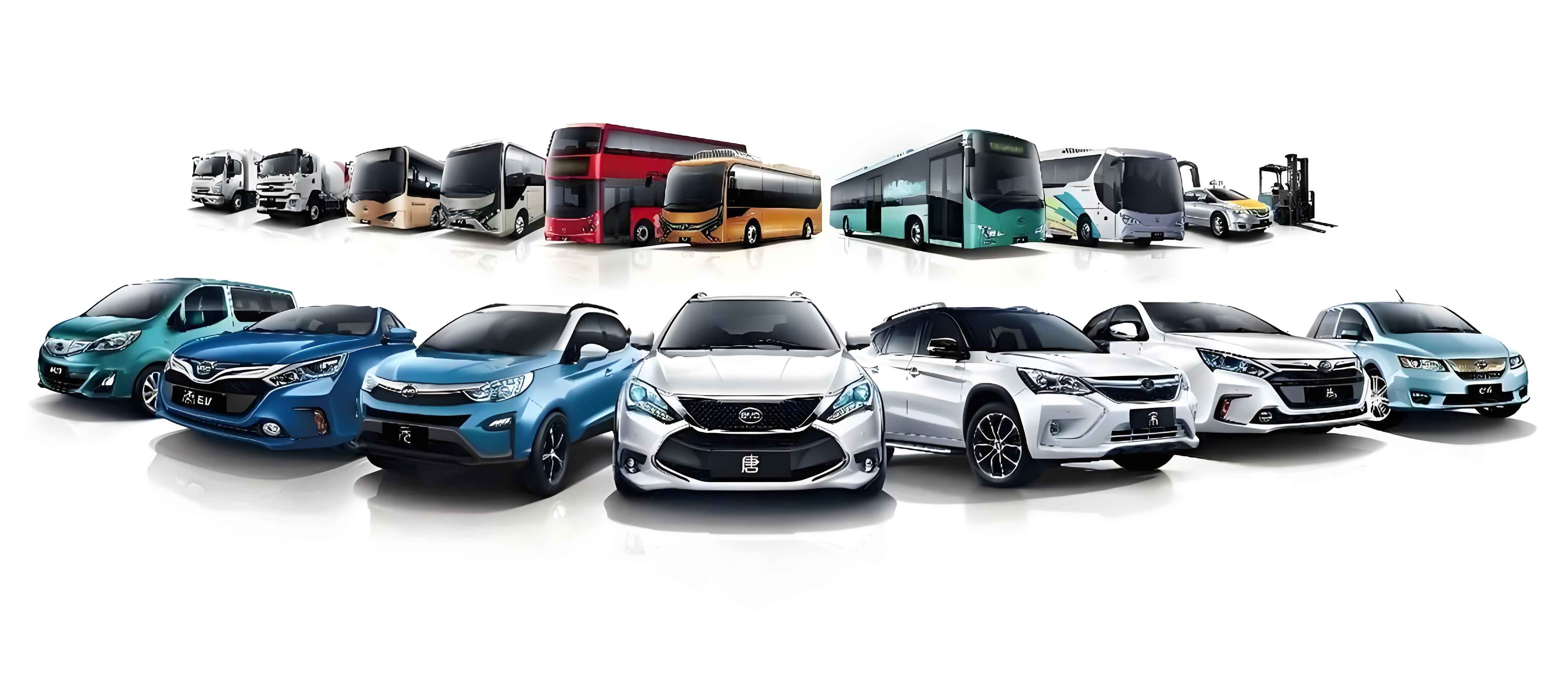
The development of the electric vehicle industry in my country has been accelerated by supportive policies, battery technology improvements, and the construction of charging infrastructure. According to recent industry statistics, electric vehicle sales exceeded 12 million units in 2024. The transition towards electric mobility is not only an industrial trend but also a strategic measure for carbon neutrality. Within the whole electric vehicle market, the distributed drive electric vehicle is catching the attention of many original equipment manufacturers because of its shortcut in the power transmission path and its superior dynamic response.
The distributed drive electric vehicle can be classified into in-wheel motor drive and wheel-side motor drive. In the in-wheel motor configuration, the motor is encapsulated inside the wheel rim. This design makes the electric vehicle structure extraordinarily compact. It also enables independent torque control on each wheel, which can create a direct yaw moment without using steering. At the same time, an in-wheel motor electric vehicle suffers from a larger unsprung mass, severe thermal management requirements, and more difficult sealing. Nevertheless, the independent control capability provided by the in-wheel motor architecture is believed to outweigh those drawbacks. Therefore, I choose the four-wheel in-wheel motor electric vehicle as the research target.
The main advantages of a distributed drive electric vehicle are summarised below. The length of the powertrain is very short because no clutch, gearbox, propeller shaft, or final drive is needed. The space utilisation of the body is increased because the motors can be integrated into the wheels. The torque response of each wheel is extremely fast, which is beneficial for electronic differential control and stability control. Moreover, one motor can continue to drive the electric vehicle after a motor failure in some redundant fault-tolerant strategies. These advantages make the distributed drive electric vehicle an ideal testbed for advanced vehicle dynamics control algorithms.
| Dimension | Permanent-magnet synchronous motor | Induction motor | Switched reluctance motor | Brushed DC motor |
|---|---|---|---|---|
| Power density (kW/kg) | 4-6 | 2-3 | 1-2 | 3-4 |
| Torque density (N·m/kg) | 20-30 | 10-15 | 15-20 | 8-12 |
| Dynamic response | Fast | Medium | Medium | Medium-fast |
| Reliability | High | Medium | Medium-high | Low |
| Cost | High | Medium | Medium-low | Low |
| Efficiency | 85%-96% | 75%-90% | 80%-90% | 70%-85% |
| Suitability for in-wheel installation | Optimal | Poor due to volume | Poor due to noise | Poor due to maintenance |
According to the above comparison, the permanent-magnet synchronous motor, or PMSM, possesses the highest torque density and a wide efficiency range. Therefore, in my research I select a surface-mounted PMSM as the wheel-hub motor. The surface-mounted PMSM has a rotor with uniformly distributed magnetic field, and its d-axis inductance is almost equal to the q-axis inductance. That property simplifies the design of vector control. In the following sections, I will introduce the PMSM model and the basic vector control strategy used in my study.
2. PMSM Modelling and Vector Control
The mathematical model of a three-phase PMSM is nonlinear and strongly coupled in the natural coordinate system. To achieve high performance, I transform the three-phase variables into a two-phase rotating reference frame. The first step is the Clark transformation from the ABC frame to the static αβ frame. The current transformation is given by
$$
\begin{bmatrix} i_\alpha \\ i_\beta \end{bmatrix}
=
\begin{bmatrix} 1 & -\frac{1}{2} & -\frac{1}{2} \\[2pt] 0 & \frac{\sqrt{3}}{2} & -\frac{\sqrt{3}}{2} \end{bmatrix}
\begin{bmatrix} i_A \\ i_B \\ i_C \end{bmatrix}.
$$
Then the Park transformation converts the αβ variables to the synchronous dq frame that rotates with the rotor. The transformation is
$$
\begin{bmatrix} i_d \\ i_q \end{bmatrix}
=
\begin{bmatrix} \cos\theta_e & \sin\theta_e \\ -\sin\theta_e & \cos\theta_e \end{bmatrix}
\begin{bmatrix} i_\alpha \\ i_\beta \end{bmatrix},
$$
where \(\theta_e\) is the electrical rotor angle. In the dq frame, the stator voltage equations of the surface-mounted PMSM can be written as
$$
\begin{aligned}
u_d &= R_s i_d + L_s \frac{\mathrm{d}i_d}{\mathrm{d}t} – \omega_e L_s i_q,\\[4pt]
u_q &= R_s i_q + L_s \frac{\mathrm{d}i_q}{\mathrm{d}t} + \omega_e L_s i_d + \omega_e \psi_f,
\end{aligned}
$$
where \(R_s\) is the stator resistance, \(L_s\) is the stator inductance, \(\omega_e\) is the electrical angular speed, and \(\psi_f\) is the flux linkage of the permanent magnet. Because I use a surface-mounted PMSM, the d-axis and q-axis inductances are assumed to be equal. The electromagnetic torque equation in the dq frame is
$$
T_e = \frac{3}{2}p\left[\psi_f i_q + \left(L_d – L_q\right)i_d i_q\right] = \frac{3}{2}p\,\psi_f i_q,
$$
since \(L_d = L_q\). This equation shows that the torque can be independently regulated by the q-axis current if the d-axis current is kept at zero. Consequently, I use the zero-d-axis-current vector control strategy.
To generate the pulse-width-modulation signals, I employ space-vector pulse-width modulation (SVPWM). The SVPWM method synthesises the desired voltage vector by combining eight basic switching states of a three-phase voltage-source inverter. In one switching period \(T_s\), the reference voltage vector \(U_{\mathrm{out}}\) is approximated by two adjacent active voltage vectors and one zero vector, as described by
$$
T_s U_{\mathrm{out}} = T_4 U_4 + T_6 U_6 + T_0 U_0 .
$$
According to the average-value equivalence principle, the duty cycles are calculated from the voltage vector angle and magnitude. The SVPWM algorithm has a higher DC-bus voltage utilisation and produces a more circular stator flux trajectory than the sinusoidal pulse-width modulation.
I built a PMSM vector-control model in MATLAB/Simulink with the parameters listed below.
| Parameter | Value |
|---|---|
| DC bus voltage | 320 V |
| Stator resistance | 0.9 Ω |
| Stator inductance | 1.7 mH |
| Nominal speed | 1100 r/min |
| Nominal power | 6 kW |
| Peak power | 15 kW |
| Rated torque | 140 N·m |
| Number of pole pairs | 4 |
| Moment of inertia | 0.0027 kg·m² |
| Damping coefficient | 0.0076 N·m·s |
The simulated speed response of the PMSM under a no-load condition tracks the reference quickly, while the startup overshoot is around 7.5% and the settling time is about 0.05 s. Under a step load, the overshoot increases to about 31% when the motor is controlled with a basic PI regulator. Since the in-wheel motor is connected directly to the wheel, any speed overshoot is reflected in a sudden wheel-speed oscillation. This phenomenon can seriously disturb the torque allocation of an electric vehicle. Therefore, it is necessary to improve the multi-motor control strategy outside the single-motor loops.
3. Improved Ring-Coupling Control for Four In-Wheel Motors
The multi-motor control problem of a distributed drive electric vehicle is more complicated than that of an ordinary industrial twin-motor system. The four in-wheel motors must track the same speed reference during the dominating straight-line motion, while they must also follow the Ackermann relationship during cornering. In practice, the load torque on each wheel motor is affected by road roughness, vertical load transfer, and side-force variations. If the speed controllers act independently, a load disturbance on one wheel will create an instantaneous speed error that cannot be sensed by the other wheels. To solve this problem, I adopt a ring-coupling topology and improve its speed-compensator design.
The conventional ring-coupling control arranges all motors in a closed chain. For the \(i\)th motor, the synchronisation error with the next motor is defined as
$$
\varepsilon_i = \omega_i – \omega_{i+1},
$$
where \(\omega_i\) is the actual speed of the \(i\)th motor, and \(\omega_{i+1}\) is the speed of the next motor in the ring. The motors are numbered 1, 2, 3, 4, and the ring is closed by comparing motor 4 with motor 1. In addition to the synchronisation error, the tracking error is defined as
$$
e_i = \omega^* – \omega_i,
$$
where \(\omega^*\) is the reference speed. In the conventional control, the two errors are combined as
$$
E_i = e_i – K_i\varepsilon_i,
$$
where the weighting factor \(K_i\) is chosen as
$$
K_i = k_0 + k_1|\varepsilon_i|,
$$
with \(k_0\) being the basic gain and \(k_1\) being the error-amplification factor. This design is straightforward but not sufficiently robust against sudden disturbances.
In my improved control strategy, I substitute the simple speed difference with a speed compensator that is based on a Fourier-series learning idea. The controller remembers the error from the previous control period and uses it to update the current compensation signal. The learning update law can be expressed as
$$
\omega_{i+1}(t) = \omega_i(t) + \Phi_i\, \mathrm{FT}\!\left(e_i(t)\right) + \Gamma_i e_i(t),
$$
where \(\Phi_i\) and \(\Gamma_i\) are adaptive learning gains. The term \(\mathrm{FT}\) represents a Fourier-series transformation of the error, which extracts periodic components from the history of the error signal. To avoid instability, I design the learning gains as
$$
\Phi_i = \Phi_{\max}\left(1 – \mathrm{e}^{-\alpha i}\right), \qquad
\Gamma_i = \Gamma_{\max}\left(1 – \mathrm{e}^{-\beta i}\right),
$$
where \(\alpha\) and \(\beta\) control the convergence rate. The parameters \(\Phi_{\max}\) and \(\Gamma_{\max}\) are selected according to the following table.
| Parameter | Range | Description |
|---|---|---|
| \(\Phi_{\max}\) | 0.1-1.0 | Feed-forward learning gain upper limit |
| \(\Gamma_{\max}\) | 0.05-0.5 | Feedback learning gain upper limit |
| \(\alpha\) | 0.05-0.2 | Increase rate of \(\Phi\) |
| \(\beta\) | 0.05-0.2 | Increase rate of \(\Gamma\) |
The stability of the learning gain is ensured by the requirement
$$
0 < \Phi_i < \frac{2J – \delta}{k_1 T_s},
$$
where \(J\) is the combined motor and wheel inertia, \(T_s\) is the sampling time, and \(\delta\) is a positive stability margin. This condition is derived using a Lyapunov function and prevents the compensation signal from diverging under repeated disturbances.
In addition to the Fourier-series learning compensator, I also introduce a proportional-integral (PI) speed compensator. The input to this compensator is the speed error between two adjacent motors. The output is the correction term \(\Delta i_q^*\) that is superimposed on the current command of the local motor. The PI compensator consists of a proportional gain \(K_p\), an integral gain \(K_i\), a nonlinear robust gain \(\mu\), and a saturation block. The discrete-time expression of the compensator is given by
$$
\begin{aligned}
u_1(k) &= K_p e(k) + K_i T_s \sum_{j=0}^{k} e(j), \\
u_2(k) &= q\,u_1(k) + \mu\,\mathrm{sgn}\left(u_1(k)\right), \\
i_q^*(k) &= \mathrm{sat}\!\left(\int u_2(k)\,\mathrm{d}t\right),
\end{aligned}
$$
where \(\mathrm{sat}\) denotes the saturation function. The nonlinear gain gives a large compensation when the speed error is high and a smooth action when the error is small, which improves the system robustness against load jumps.
Figure 1 shows the architecture of an improved ring-coupling control system that I built for four in-wheel motors. The four motor models have their own vector-control loops. In addition, the measured speeds are exchanged through the ring structure, and the speed compensator generates the compensatory current signals. Moreover, I add an external load torque input to each motor model so that I can simulate non-symmetric disturbances that occur on a real electric vehicle.
I compared three control structures in MATLAB/Simulink: the conventional ring-coupling control, the deviation-coupling control, and the improved ring-coupling control. The reference speed was 800 r/min for all four motors. The speed responses under a no-load starting condition are summarised in the following table.
| Control strategy | Rise time (s) | Peak speed (r/min) | Overshoot (%) | Settling time (s) |
|---|---|---|---|---|
| Conventional ring coupling | 0.015 | 840 | 5.0 | 0.04 |
| Deviation coupling | 0.012 | 890 | 11.3 | 0.06 |
| Improved ring coupling | 0.015 | 830 | 3.75 | 0.035 |
The improved ring-coupling control yields the smallest overshoot and the shortest settling time among the three methods. Compared with the deviation-coupling method, the overshoot is reduced by about 7.6%, and the settling time is shortened by about 41.7%. This result confirms that the speed compensator can effectively suppress the transient overshoot without sacrificing response speed, which is of great significance for an in-wheel motor electric vehicle.
I further tested the disturbance response by applying a load torque change to motor 1 and motor 2 at \(t=0.5\) s while the remaining motors kept a constant load. The maximum tracking errors observed with the three strategies are summarised in the table below.
| Indicator | Conventional ring coupling | Deviation coupling | Improved ring coupling |
|---|---|---|---|
| Maximum error of motor 1 (r/min) | 65 | 60 | 60 |
| Maximum error of motor 2 (r/min) | 35 | 35 | 25 |
| Maximum error of motor 3 (r/min) | 20-35 | 15 | 10 |
| Maximum error of motor 4 (r/min) | 20-35 | 15 | 10 |
| Error distribution | Non-uniform | Moderate | Most uniform |
| Recovery time to \(\pm5\) r/min (s) | 0.03 | 0.025 | 0.02 |
From the table, the improved ring-coupling control has the best capability to equalise the errors among the four motors. When motors 3 and 4 are exposed to a disturbance that is transferred through the coupling chain, the maximum error stays below 10 r/min, whereas the conventional method produces errors between 20 and 35 r/min. The improved structure therefore suppresses the propagation of the error along the ring and shortens the recovery time. This property is essential for a distributed drive electric vehicle that travels on roads with changing friction coefficients.
4. Vehicle Dynamics Reference Model
After designing the motor-level synchronisation control, I turn to the vehicle-level stability control. A common method is to use direct yaw-moment control, in which an extra yaw moment is added around the vertical axis of the electric vehicle. To calculate the required yaw moment, I need a reference model that represents the desired handling behaviour. The linear two-degree-of-freedom (2-DOF) bicycle model is widely used because of its simplicity and real-time capability. In this model, the vehicle state variables are the sideslip angle \(\beta\) and the yaw rate \(\gamma\). The equations of motion are given by
$$
\begin{aligned}
m v_x\left(\dot{\beta} + \gamma\right) &= F_{y1} + F_{y2}, \\
I_z \dot{\gamma} &= a F_{y1} – b F_{y2},
\end{aligned}
$$
where \(m\) is the vehicle mass, \(v_x\) is the longitudinal velocity, \(I_z\) is the yaw moment of inertia, \(a\) is the distance from the centre of gravity to the front axle, and \(b\) is the distance to the rear axle. The lateral tyre forces \(F_{y1}\) and \(F_{y2}\) can be expressed as linear functions of the tyre slip angles when the lateral acceleration is not too high:
$$
F_{y1} = k_f \alpha_1, \qquad F_{y2} = k_r \alpha_2,
$$
where \(k_f\) and \(k_r\) are the equivalent cornering stiffness values of the front and rear axles, and \(\alpha_1\), \(\alpha_2\) are the corresponding slip angles. Assuming a small front steering angle \(\delta\), the state-space representation becomes
$$
\dot{x} = A x + B \delta,
$$
with \(x=[\beta,\gamma]^\mathrm{T}\) and
$$
A =
\begin{bmatrix}
\dfrac{k_f+k_r}{m v_x} & \dfrac{a k_f – b k_r}{m v_x^2} – 1 \\[8pt]
\dfrac{a k_f – b k_r}{I_z} & \dfrac{a^2 k_f + b^2 k_r}{I_z v_x}
\end{bmatrix},
\qquad
B =
\begin{bmatrix}
-\dfrac{k_f}{m v_x} \\[6pt]
-\dfrac{a k_f}{I_z}
\end{bmatrix}.
$$
For steady-state cornering, the derivatives of \(\beta\) and \(\gamma\) are zero. Therefore, the desired yaw rate and the desired sideslip angle can be written as
$$
\gamma_d = \frac{v_x / L}{1 + K v_x^2}\,\delta,
$$
$$
\beta_d = \frac{b – \frac{m a v_x^2}{k_r L}}{L\left(1 + K v_x^2\right)}\,\delta,
$$
where \(L=a+b\) is the wheelbase and \(K\) is the stability factor defined by
$$
K = \frac{m}{L^2}\left(\frac{a}{k_r} – \frac{b}{k_f}\right).
$$
The desired values must be constrained by the road friction coefficient \(\mu\). I used the following limits:
$$
|\gamma_d| \le \frac{0.85 \mu g}{v_x}, \qquad |\beta_d| \le \arctan(0.02 \mu g),
$$
where \(g\) is the acceleration due to gravity. These constraints prevent the reference values from demanding unreachable lateral acceleration on low-friction roads.
In my vehicle control architecture, the upper layer calculates the difference between the actual yaw rate and the desired yaw rate. The error is fed to a yaw-moment controller, which outputs the additional yaw moment \(\Delta M\). The lower layer then distributes the driving torque among the four in-wheel motors. This layered structure is easy to tune and offers a clear separation between the decision stage and the allocation stage.
5. Upper-Layer Yaw-Moment Controllers
5.1 Traditional PI controller
The simplest yaw-moment controller is a proportional-integral (PI) controller. The control law is
$$
\Delta M = K_p e_\gamma + K_i \int e_\gamma \,\mathrm{d}t,
$$
where \(e_\gamma = \gamma – \gamma_d\). I tuned the gains by following the classical trial-and-error procedure. First, I disabled the integral part and increased the proportional gain until the response became sufficiently fast but did not oscillate. Then, I gradually added the integral gain to remove the steady-state yaw-rate error. The PI controller is stable and effective for a large range of operating conditions, but its fixed gains cannot adapt to changes in vehicle speed, road friction, and tyre nonlinearity. Hence, I also investigated a fuzzy PID controller for the same purpose.
5.2 Fuzzy PID controller
A fuzzy PID controller adjusts the three gains \(K_p\), \(K_i\), and \(K_d\) online according to the control error \(e\) and the derivative of the error \(\mathrm{d}e/\mathrm{d}t\). In my design, the inputs to the fuzzy inference system are the yaw-rate error \(E\) and the error change rate \(EC\). The output variables are the increments \(\Delta K_p\), \(\Delta K_i\), and \(\Delta K_d\). The actual gains used in the PID law are
$$
K_p = K_{p0} + \Delta K_p, \qquad
K_i = K_{i0} + \Delta K_i, \qquad
K_d = K_{d0} + \Delta K_d.
$$
I selected seven fuzzy sets for both inputs and outputs: NB, NM, NS, ZO, PS, PM, and PB. The membership functions of the inputs are triangular-shaped, and the defuzzification method is the centre of gravity. The fuzzy rules follow the conventional principle known from vehicle stability control.
When the yaw-rate error is negative large and the error change is negative large, the system is deviating rapidly from the desired yaw rate. In this case, I increase the proportional gain and the derivative gain while decreasing the integral gain, which forces the controller to react promptly and suppresses the overshoot. When the yaw-rate error is near zero and its change rate is also near zero, I keep the derivative gain small to avoid sensitivity to measurement noise and increase the integral gain to remove steady-state error. The following tables list the fuzzy rule matrices for \(\Delta K_p\), \(\Delta K_i\), and \(\Delta K_d\).
| \(E\) \ \(EC\) | NB | NM | NS | ZO | PS | PM | PB |
|---|---|---|---|---|---|---|---|
| NB | PB | PB | PM | PM | PS | ZO | ZO |
| NM | PB | PM | PM | PS | ZO | NS | NS |
| NS | PM | PM | PS | ZO | NS | NM | NM |
| ZO | PM | PS | ZO | ZO | ZO | NS | NM |
| PS | PS | ZO | NS | ZO | NS | NM | NM |
| PM | ZO | NS | NM | NS | NM | NM | NB |
| PB | ZO | NS | NM | NM | NM | NB | NB |
| \(E\) \ \(EC\) | NB | NM | NS | ZO | PS | PM | PB |
|---|---|---|---|---|---|---|---|
| NB | NB | NB | NM | NM | NS | ZO | ZO |
| NM | NB | NM | NM | NS | ZO | ZO | PS |
| NS | NM | NM | NS | ZO | PS | PS | PM |
| ZO | NM | NS | ZO | PM | ZO | NS | NM |
| PS | NS | ZO | PS | ZO | NS | NM | NM |
| PM | ZO | ZO | PS | NS | NM | NM | NB |
| PB | ZO | NS | NM | NM | NB | NB | NB |
| \(E\) \ \(EC\) | NB | NM | NS | ZO | PS | PM | PB |
|---|---|---|---|---|---|---|---|
| NB | PS | PM | PB | PB | PM | PS | ZO |
| NM | PM | PB | PB | PM | PS | ZO | NS |
| NS | PB | PB | PM | PS | ZO | NS | NM |
| ZO | PB | PM | PS | ZO | PS | PM | PB |
| PS | NM | NS | ZO | PS | PM | PB | PB |
| PM | NS | ZO | PS | PM | PB | PB | PM |
| PB | ZO | PS | PM | PB | PB | PM | PS |
The fuzzy inference rules are evaluated with the Mamdani algorithm, and the centre of gravity is used in defuzzification. The resulting gain surface is continuous and monotonic in each region, which provides a smooth transition between the control actions.
6. Lower-Layer Torque Distribution
Once the upper layer gives the total driving force demand \(F_d\) and the additional yaw moment \(\Delta M\), the lower layer must allocate the four wheel torques \(T_{ij}\). My distribution law is based on the static load ratio between the front and rear axles. The vertical loads of the front and rear axles under longitudinal acceleration \(a_x\) are
$$
F_{zf} = \frac{mgb – m a_x h_g}{L}, \qquad
F_{zr} = \frac{mga + m a_x h_g}{L},
$$
where \(h_g\) is the height of the centre of gravity. The wheel-drive-force allocation must satisfy the total traction:
$$
F_{x11} + F_{x12} + F_{x21} + F_{x22} = F_d,
$$
and the yaw-moment allocation:
$$
\frac{B}{2}\left(F_{x12} – F_{x11}\right) + \frac{B}{2}\left(F_{x22} – F_{x21}\right) = \Delta M,
$$
where \(B\) is the track width and the subscript 11 denotes front-left, 12 front-right, 21 rear-left, and 22 rear-right. I distribute the total force between the two axles proportionally to the axle-load ratio:
$$
\frac{F_{x11} + F_{x12}}{F_{x21} + F_{x22}} = \frac{F_{zf}}{F_{zr}}.
$$
By combining the previous equations, I obtain the longitudinal forces on each wheel. The wheel torque is then simply
$$
T_{ij} = R\,F_{xij},
$$
where \(R\) is the tyre rolling radius. The final torque commands are limited by the motor maximum torque and the road friction capability. This lower-layer controller naturally provides more driving torque to the axle with a larger vertical load, which increases the tyre utilisation margin during acceleration or deceleration.
The table below summarises the strategy for correcting understeer and oversteer conditions on an in-wheel motor electric vehicle.
| Steering direction | Stability condition | Target yaw moment | Outer wheels | Inner wheels |
|---|---|---|---|---|
| Left turn | Understeer | \(\Delta M>0\) | Increase torque | Decrease torque |
| Left turn | Oversteer | \(\Delta M<0\) | Decrease torque | Increase torque |
| Right turn | Understeer | \(\Delta M<0\) | Decrease torque | Increase torque |
| Right turn | Oversteer | \(\Delta M>0\) | Increase torque | Decrease torque |
The direct yaw-moment control based on torque allocation is often called torque-vectoring control. It is especially attractive for a distributed drive electric vehicle because every wheel can generate either a positive traction force or a negative regenerative force. Therefore, a corrective yaw moment can be produced without reducing the total driving force.
7. Co-Simulation Environment and Results
I verified the proposed control strategy by using a high-fidelity vehicle dynamics software, CarSim, combined with MATLAB/Simulink. The CarSim model provides tyre nonlinearities, suspension kinematics, and realistic road conditions. I modified the default vehicle model to remove its internal combustion engine, gearbox, and differential. Instead, I selected the ‘four-wheel-drive’ configuration with “All External Powertrain Components”. In this way, the driving torque of each wheel in the virtual electric vehicle is directly supplied by my Simulink controller.
The main parameters of the simulated electric vehicle are shown in the table below.
| Parameter | Value |
|---|---|
| Curb mass (kg) | 1270 |
| Wheelbase (mm) | 2910 |
| Distance from CG to front axle (mm) | 1015 |
| Distance from CG to rear axle (mm) | 1895 |
| Front track width (mm) | 1675 |
| Rear track width (mm) | 1675 |
| CG height (mm) | 540 |
| Tyre rolling radius (mm) | 325 |
| Front axle cornering stiffness (N/rad) | -52395 |
| Rear axle cornering stiffness (N/rad) | -34510 |
| Wheel moment of inertia (kg·m²) | 0.8 |
I first tested the vehicle behaviour under a fast double-lane-change manoeuvre on a road with a friction coefficient of 0.5. The vehicle speed was kept at 90 km/h. Three control configurations were compared: no upper-layer control, conventional PI control, and fuzzy PID control. The lateral displacement of the vehicle’s centre of gravity was recorded to evaluate path-following ability.
The path-following performance is summarised in the following table.
| Indicator | No control | PI control | Fuzzy PID control |
|---|---|---|---|
| Peak lateral displacement error relative to reference (%) | 17 | 10 | 6 |
| Vehicle speed during cornering (km/h) | Not reduced | Reduced to 85-88 | Reduced to 87-88 |
| Yaw-rate tracking | Large oscillation | Medium oscillation | Small oscillation |
| Sideslip angle peak (°) | Large | Moderate | Small |
These results show that the fuzzy PID controller reduces the path deviation by more than 60% compared with the no-control case. It also improves the yaw-rate tracking and decreases the vehicle sideslip angle. In the speed response, the fuzzy PID controller proactively reduces the vehicle speed during the high-lateral-acceleration section and then recovers to the target speed, which helps to avoid unstable cornering.
I then tested the fuzzy PID controller in a double-lane change with an abrupt friction change from 0.8 to 0.4 and back to 0.8. The vehicle speed was again 90 km/h. In this case, the momentum of the electric vehicle tends to excite severe sideslip when the tyres lose grip. The fuzzy PID controller maintains a good tracking of the reference path and limits the sideslip angle to a small range. The yaw rate oscillation is obvious only within the low-friction interval, but it decays quickly after the vehicle returns to the high-friction surface.
I also examined an open-friction road, where the left wheel track has a friction coefficient of 0.8 while the right wheel track has 0.4. This is one of the most difficult operating conditions for a distributed drive electric vehicle because the brake or drive forces on the two sides are highly asymmetrical. In this scenario, the fuzzy PID controller still guarantees the stability of the vehicle, although the maximum sideslip angle is larger than that of the front-back friction-change scenario. The yaw-rate peak is increased in the low-friction interval, but no instability occurs.
After verifying the upper-layer decision, I integrated the improved ring-coupling control structure from Section 3 into the vehicle-level simulation. In this integrated scheme, the upper layer still generates the additional yaw moment using fuzzy PID, while the lower layer outputs the individual wheel torque commands. The four in-wheel motors are synchronised with the improved ring-coupling strategy. I observed the wheel-speed responses and the vehicle states during the fast double-lane change on μ=0.5. The wheel-speed simulation results are described below.
When the electric vehicle was controlled only by the fuzzy PID unit without the ring-coupling structure, the left and right rear-wheel speeds exhibited visible oscillations around the target values. The peak of the speed oscillation occurred in different time instants for different wheels. After the improved ring-coupling structure was added, the wheel-speed curves became more consistent. The synchronisation error between the left and right rear wheels was substantially reduced. This improvement indicates that the ring-coupling control can assist the yaw-moment controller by preventing individual wheel slip and excessive wheel-speed differences.
The benefits of combining the fuzzy PID controller and the improved ring-coupling control are quantified in the following table.
| Indicator | No control | Fuzzy PID without ring coupling | Fuzzy PID + improved ring coupling |
|---|---|---|---|
| Peak lateral displacement error (%) | 17 | 6 | 4 |
| Peak sideslip angle (°) | >1.20 (unstable region) | 0.85 | 0.70 |
| Yaw-rate error | Large | Medium | Smallest |
| Wheel-speed oscillation | Large | Medium | Small |
From these simulation results, the integrated controller can reduce the peak lateral displacement error to 4%, while the sideslip angle is reduced from 0.85° with fuzzy PID alone to 0.70° with the proposed integrated strategy. The sideslip angle remains within the commonly cited safe range of ±2.5° throughout the manoeuvre. The yaw rate follows the desired value more closely in all phases of the double-lane change.
In addition to the double-lane change, I performed a sinusoidal steering input test at 90 km/h to assess the dynamic response of the electric vehicle. The fuzzy PID controller in combination with the improved ring-coupling structure effectively suppresses the amplitude deviation of the yaw rate and reduces the phase lag between the actual yaw rate and the desired yaw rate. Without the coupling structure, the rear wheels tend to oscillate after the steering direction is reversed, which produces a fatiguing behaviour for the driver. The proposed controller has a significant smoothing effect on those oscillations.
8. Discussion of Control Complexity and Real-Time Implementation
One important issue in an electric vehicle control system is the computational cost of the algorithm. The non-coupled multi-motor control method has the lowest complexity, but it cannot suppress synchronisation errors. The coupled ring-coupling methods increase the computational cost only slightly because each motor communicates with at most two neighbouring motors. Table below compares the computational complexity of several control algorithms used in electric vehicle motor systems.
| Algorithm | Typical operations per control period | Time complexity | Practical applicability |
|---|---|---|---|
| PI | 5-8 basic operations | \(O(1)\) | Very high |
| Sliding mode | 20-30 basic operations | \(O(1)\) | High but with chattering |
| Fuzzy PID | 50-100 basic operations | \(O(m)\) (\(m\)=49 rules) | High |
| Adaptive control | 20-50 operations with parameter updates | \(O(p^2)\) | Medium |
| Model predictive control | 100-1000 floating-point operations | \(O(n^3)\) | Requires powerful processor |
The proposed improved ring-coupling control adds only a small number of arithmetic operations to the local PI current loops. The Fourier-series transformation is based on the current and previous error values; therefore, its memory footprint is limited. The fuzzy PID controller also has a fixed number of rules, which means that its execution time is deterministic. As a result, the combined control strategy is suitable for an embedded controller in a practical in-wheel motor electric vehicle.
From the perspective of the electric vehicle dynamics, the use of the improved ring-coupling control at the motor level offers a natural tolerance to wheel-speed disagreement. It reduces the reliance on the yaw-moment controller to compensate for motor-speed ripples. The hierarchical controller can therefore focus on the vehicle’s global lateral and longitudinal motion, while the motor-level controller preserves the wheel-speed synchronisation. This separation of responsibilities is beneficial for hardware-in-the-loop testing and future vehicle deployment.
9. Conclusion
In this work, I investigated the control strategy of an in-wheel motor in a distributed drive electric vehicle. I first developed a PMSM vector-control model and identified the limitations of the independent motor control in a multi-motor powertrain. I then proposed an improved ring-coupling control strategy that utilises a Fourier-series speed-compensator and a nonlinear PI compensator. The simulation results demonstrated that the proposed strategy reduces the synchronisation error among four in-wheel motors and shortens the error-recovery time under non-symmetric load disturbances.
At the vehicle level, I established a hierarchical control architecture for a four-wheel in-wheel motor electric vehicle. The upper layer uses a fuzzy PID controller that generates the additional yaw moment from the yaw-rate error and the sideslip-angle error. The lower layer distributes torque according to the front-rear axle load ratio. The performance of the fuzzy PID controller was compared with that of the traditional PI controller and a no-control scheme in CarSim. The fuzzy PID controller gave a smaller path-tracking error, a lower peak sideslip angle, and better yaw-rate tracking than the conventional PI controller.
Finally, I merged the improved ring-coupling control with the fuzzy PID yaw-moment control and tested the integrated strategy in a high-speed double-lane-change manoeuvre with a low friction coefficient. The integrated controller achieved a peak lateral displacement error of only 4%, reduced the sideslip angle by 17.65% compared with fuzzy PID alone, and substantially suppressed the wheel-speed oscillations. These results confirm that the combination of motor-level synchronisation control and vehicle-level torque-vectoring control is a promising solution for the next-generation distributed drive electric vehicle.
Future research directions may include the following aspects. First, I plan to extend the study to extreme driving conditions such as snowy roads and split-friction surfaces, where road friction estimation is essential. Second, an energy-optimal torque distribution algorithm can be added to the lower layer to minimise the total electrical energy consumption of the electric vehicle while maintaining the stability performance. Third, hardware-in-the-loop experiments and real-vehicle tests can be carried out to validate the real-time feasibility of the control code. With the continuous development of electric vehicle technology, I believe that in-wheel motor control strategies will become an important enabler for safer and more efficient future vehicles.