
I propose an intelligent fault diagnosis method for electric vehicle charging piles by integrating a convolutional neural network, a bidirectional long short-term memory network, and an attention mechanism. The motivation is straightforward: electric vehicle charging piles are safety-critical assets in modern charging infrastructure, and their failure rates remain high because of complex power electronics, communication modules, locking devices, environmental stress, and continuous high-load operation. In my view, accurate and automated diagnosis of electric vehicle charging pile faults is essential for reducing maintenance cost, improving service reliability, and preventing safety incidents. The model I develop in this article processes electric vehicle charging pile data through missing-value imputation, outlier removal, and normalization, then extracts local patterns with a CNN, captures temporal dependencies with a BiLSTM network, and reweights informative representations with an attention module. I evaluate the method on a public electric vehicle charging pile fault classification dataset and compare it with several baseline models. The experimental results show that the proposed model achieves an average accuracy of 0.91, which is 0.17 higher than BiLSTM and 0.07 higher than CNN-BiLSTM. I also provide detailed formulations, parameter tables, and ablation-style comparisons to make the design reproducible and to clarify why the combination of local feature extraction, bidirectional temporal modeling, and attention-based weighting is effective for electric vehicle charging pile fault diagnosis.
1. Introduction
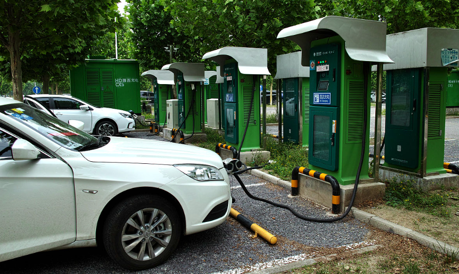
Electric vehicle charging infrastructure has expanded rapidly, and electric vehicle charging piles have become one of the most important interfaces between transportation systems and power grids. A fault in an electric vehicle charging pile can interrupt charging service, increase operation and maintenance costs, damage user confidence, and in severe cases create fire hazards or grid-side disturbances. Common electric vehicle charging pile faults include power module overheating, communication abnormalities, insulation failures, emergency-stop misoperations, electronic-lock failures, door-access anomalies, and harmonic distortion problems. Because these faults may appear as subtle deviations in multi-channel signals, manual inspection and rule-based alarm logic are often insufficient for large-scale electric vehicle charging pile fleets.
I observe that traditional diagnosis approaches for electric vehicle charging piles usually rely on human inspection, threshold checking, or analytical models. Such methods can be effective for isolated cases, but they are difficult to scale and often suffer from low accuracy under noisy operating conditions. Machine learning methods can improve diagnostic accuracy and fuse multiple signal sources, but they may depend heavily on high-quality labeled data and carefully engineered features. Deep learning methods offer a different route: they can learn hierarchical representations directly from electric vehicle charging pile data and can model nonlinear relationships among multiple sensor channels. Nevertheless, a single CNN or a single recurrent network may not fully exploit both local signal morphology and long-range temporal context. This is the gap that motivates my CNN-BiLSTM-Attention model for electric vehicle charging pile fault diagnosis.
The main contributions I make in this article are as follows. First, I design a multi-scale CNN front end for electric vehicle charging pile signals, where one-dimensional convolution kernels of different sizes capture local transient patterns and short-term waveform variations. Second, I use a two-layer BiLSTM to model forward and backward temporal dependencies in electric vehicle charging pile sequences, which improves the utilization of contextual information compared with a unidirectional LSTM. Third, I introduce an attention mechanism that assigns different weights to different positions in the sequence, allowing the model to focus on fault-relevant segments and suppress irrelevant fluctuations. Fourth, I report a systematic experimental comparison on an electric vehicle charging pile fault dataset, including average accuracy, minimum accuracy, maximum accuracy, and ablation-style comparisons. The results confirm that the proposed model provides higher diagnostic accuracy for electric vehicle charging pile faults and offers a practical reference for intelligent operation and maintenance.
2. Problem Formulation and Data Description
I formulate electric vehicle charging pile fault diagnosis as a supervised binary classification problem. For each electric vehicle charging pile sample, the input is a multivariate time-series segment with six measured channels, and the output is a label indicating whether the electric vehicle charging pile is in a normal state or an abnormal state. Let the input sequence be
$$ X = [x_1, x_2, \ldots, x_T] \in \mathbb{R}^{T \times M}, $$
where \(T\) is the sequence length, \(M\) is the number of input features, and \(x_t \in \mathbb{R}^{M}\) denotes the feature vector at time step \(t\). In this study, \(M=6\) for the measured channels, and the label is binary. I denote the label as \(y \in \{0,1\}\), where \(0\) corresponds to a normal electric vehicle charging pile state and \(1\) corresponds to an abnormal electric vehicle charging pile state. The goal is to learn a mapping
$$ f_{\theta}: \mathbb{R}^{T \times M} \rightarrow \{0,1\}, $$
where \(\theta\) denotes the trainable parameters of the CNN-BiLSTM-Attention model. The dataset used in my experiments contains six features and a binary label. The features are the K1K2 drive signal, the electronic-lock drive signal, the emergency-stop signal, the door-access signal, the total voltage harmonic distortion signal, and the total current harmonic distortion signal. The label value “1” indicates a normal electric vehicle charging pile state, and the label value “2” indicates an abnormal electric vehicle charging pile state. For modeling convenience, I map these labels to 0 and 1 during training and map them back during interpretation. Each feature contains 85,500 data points, and the normal and abnormal states are approximately balanced at 50% each. This balance reduces the risk of trivial majority-class prediction and makes accuracy a meaningful primary metric for electric vehicle charging pile fault diagnosis.
| Feature index | Feature name | Physical meaning in electric vehicle charging pile operation | Role in fault diagnosis |
|---|---|---|---|
| 1 | K1K2 drive signal | Controls the start-up and locking sequence of the electric vehicle charging process. | Indicates whether the electric vehicle charging pile can initiate and latch the charging procedure correctly. |
| 2 | Electronic-lock drive signal | Supports safety locking, physical connection confirmation, and fault protection. | Reflects connector engagement and locking reliability of the electric vehicle charging pile. |
| 3 | Emergency-stop signal | Cuts off power immediately under operator error, fault, or emergency conditions. | Captures emergency protection behavior and possible misoperation of the electric vehicle charging pile. |
| 4 | Door-access signal | Provides identity verification and authorization for safe access. | Reflects access-control anomalies and unauthorized opening events of the electric vehicle charging pile. |
| 5 | THDV-M | Total voltage harmonic distortion measurement. | Indicates voltage waveform distortion that may destabilize the electric vehicle charging pile and the grid. |
| 6 | THDI-M | Total current harmonic distortion measurement. | Indicates current distortion that may increase losses and reduce power factor in electric vehicle charging operation. |
| 7 | Label | Binary state label of the electric vehicle charging pile. | 1 denotes normal state; 2 denotes abnormal state in the original dataset. |
The six channels are heterogeneous. Some are discrete or quasi-discrete drive signals, while others are continuous harmonic-distortion measurements. The numerical ranges also differ considerably. For this reason, I treat preprocessing as a first-class part of the pipeline rather than an optional step. If I feed raw electric vehicle charging pile signals directly into a deep network, the model may be dominated by large-magnitude channels and may fail to learn subtle but diagnostically important patterns in smaller-magnitude channels. I therefore apply missing-value imputation, outlier processing, and standardization before training.
3. Data Preprocessing
I organize the preprocessing of electric vehicle charging pile data into four steps: missing-value imputation, outlier handling, normalization, and dataset partitioning. The purpose is to ensure data integrity, numerical stability, and fair model comparison. Missing values can arise from sensor dropouts, communication interruptions, or data storage issues in electric vehicle charging pile monitoring systems. I use mean imputation for each feature so that the filled value remains consistent with the central tendency of the corresponding channel. Let \(A_{ij}\) be the \(i\)-th observed value of feature \(j\), and let \(\beta_{ij}\in\{0,1\}\) be an indicator that equals 1 when the value is missing and 0 otherwise. The imputed value is
$$ \hat{A}_{j} = \frac{1}{n_j}\sum_{i=1}^{n_j}\beta_{ij} A_{ij}, $$
where \(n_j\) is the number of missing entries considered for feature \(j\). In implementation, I compute the mean from the available observations of the same feature and replace missing entries with that mean. This simple strategy preserves the sample size and avoids introducing strong bias from arbitrary constant filling.
For outlier handling, I adopt the three-sigma rule. For each feature, I estimate the mean \(\mu_j\) and standard deviation \(\sigma_j\), and I flag a value \(x_{ij}\) as an outlier when
$$ |x_{ij}-\mu_j| > 3\sigma_j. $$
I remove or replace such values according to the preprocessing policy. The three-sigma criterion is suitable for electric vehicle charging pile signals because most normal operating measurements cluster around a stable mean, while extreme values often correspond to sensor faults, communication errors, or transient disturbances. Removing these extreme outliers prevents the network from overfitting to non-physical spikes.
After outlier handling, I standardize each feature to zero mean and unit variance. The normalization formula is
$$ z_{ij} = \frac{x_{ij}-\mu_j}{\sigma_j}, $$
where \(z_{ij}\) is the normalized value, \(x_{ij}\) is the original value, \(\mu_j\) is the feature mean, and \(\sigma_j\) is the feature standard deviation. This step eliminates unit differences among the six electric vehicle charging pile channels and makes gradient-based optimization more stable. I then shuffle the samples and split the dataset into 80% training, 10% validation, and 10% test subsets. The validation subset is used for model selection and early stopping, while the test subset is reserved for final evaluation. I repeat each experiment ten times to reduce the influence of random initialization and data splitting.
| Step | Operation | Formula or rule | Purpose |
|---|---|---|---|
| 1 | Missing-value imputation | \(\hat{A}_{j}=\frac{1}{n_j}\sum_{i=1}^{n_j}\beta_{ij}A_{ij}\) | Preserve sample size and data continuity for electric vehicle charging pile diagnosis. |
| 2 | Outlier detection | \(|x_{ij}-\mu_j|>3\sigma_j\) | Remove non-physical spikes and measurement errors. |
| 3 | Normalization | \(z_{ij}=(x_{ij}-\mu_j)/\sigma_j\) | Eliminate scale differences among electric vehicle charging pile channels. |
| 4 | Dataset partitioning | 80% training, 10% validation, 10% test | Support fair training, model selection, and final evaluation. |
4. CNN-BiLSTM-Attention Model
The overall architecture I design contains five functional stages: input representation, multi-scale CNN feature extraction, BiLSTM temporal modeling, attention-based weighting, and fully connected classification. The input is an \(N \times M\) matrix, where \(N\) is the number of time-series training samples and \(M\) is the feature dimension at each time point. In this work, \(M=7\) when the binary label is included in the tabular description, while the model input itself uses the six measured electric vehicle charging pile channels and treats the label as the supervised target. The CNN front end contains two one-dimensional convolution branches with kernel sizes \(3\times 1\) and \(5\times 1\), respectively, followed by batch normalization, ReLU activation, and dropout. The two branches are fused by a \(1\times 1\) convolution with 256 feature maps. The BiLSTM stage contains two layers with hidden dimensions 128 and 64. The attention stage computes a weighted sum over the BiLSTM outputs. The classifier contains three fully connected layers with 128, 64, and the final number of classes, respectively. I use softmax and cross-entropy loss for training.
4.1 Multi-Scale CNN for Local Feature Extraction
A CNN is effective for extracting local patterns from electric vehicle charging pile signals because convolution kernels act as learnable local filters. In my design, the multi-scale front end uses two parallel one-dimensional convolution branches. The small kernel of size 3 captures short local transients, while the larger kernel of size 5 captures slightly broader waveform patterns. This is important for electric vehicle charging pile diagnosis because some faults appear as abrupt switching anomalies, whereas others appear as sustained harmonic distortion or gradual drift. Let \(X\) be the input sequence. The two branches are computed as
$$ H_3 = \mathrm{Dropout}\left(\mathrm{ReLU}\left(\mathrm{BN}\left(W_3 * X + b_3\right)\right)\right), $$
$$ H_5 = \mathrm{Dropout}\left(\mathrm{ReLU}\left(\mathrm{BN}\left(W_5 * X + b_5\right)\right)\right), $$
where \(*\) denotes one-dimensional convolution, \(W_3\) and \(W_5\) are convolution kernels of sizes 3 and 5, \(b_3\) and \(b_5\) are biases, \(\mathrm{BN}\) denotes batch normalization, and \(\mathrm{ReLU}\) is the rectified linear unit. I set the number of feature maps to 128 in each branch and the dropout rate to 0.2. The fused representation is
$$ H_f = \mathrm{Dropout}\left(\mathrm{ReLU}\left(\mathrm{BN}\left(W_1 * [H_3;H_5] + b_1\right)\right)\right), $$
where \(W_1\) is a \(1\times 1\) convolution with 256 feature maps, and \([H_3;H_5]\) denotes channel concatenation. The \(1\times 1\) convolution fuses multi-scale information and projects it into a compact representation for the recurrent stage. Batch normalization introduces mild noise during training, reduces sensitivity to initialization, and improves the robustness of electric vehicle charging pile fault diagnosis under varying signal scales. Dropout at rates 0.2 and 0.3 mitigates overfitting.
| Component | Kernel size | Number of feature maps | Stride | Activation | Dropout | Function |
|---|---|---|---|---|---|---|
| Branch 1 convolution | \(3\times 1\) | 128 | 1 | ReLU | 0.2 | Capture short local transients in electric vehicle charging pile signals. |
| Branch 2 convolution | \(5\times 1\) | 128 | 1 | ReLU | 0.2 | Capture broader local waveform patterns. |
| Fusion convolution | \(1\times 1\) | 256 | 1 | ReLU | 0.3 | Fuse multi-scale features and project to recurrent input. |
4.2 BiLSTM for Temporal Dependency Modeling
Electric vehicle charging pile signals are sequential. A fault may manifest not only as a local spike but also as a temporal pattern, such as a delayed lock response, a repeated emergency-stop sequence, or a gradual increase in harmonic distortion. A unidirectional LSTM can model past context, but it cannot use future context within the same window. BiLSTM solves this limitation by running two LSTM directions and concatenating their hidden states. For an input sequence \(x_t\), the forward LSTM produces \(\overrightarrow{h}_t\) and the backward LSTM produces \(\overleftarrow{h}_t\). The concatenated representation is
$$ h_t = [\overrightarrow{h}_t;\overleftarrow{h}_t]. $$
The internal LSTM gates are computed as follows:
$$ f_t = \sigma\left(W_f[h_{t-1},x_t]+b_f\right), $$
$$ i_t = \sigma\left(W_i[h_{t-1},x_t]+b_i\right), $$
$$ \tilde{C}_t = \tanh\left(W_C[h_{t-1},x_t]+b_C\right), $$
$$ C_t = f_t\odot C_{t-1}+i_t\odot\tilde{C}_t, $$
$$ o_t = \sigma\left(W_o[h_{t-1},x_t]+b_o\right), $$
$$ h_t = o_t\odot\tanh(C_t), $$
where \(f_t\), \(i_t\), and \(o_t\) are the forget, input, and output gates, respectively; \(C_t\) is the cell state; \(\tilde{C}_t\) is the candidate cell state; \(\sigma\) is the sigmoid function; \(\odot\) denotes element-wise multiplication; and \(W_f,W_i,W_C,W_o\) and \(b_f,b_i,b_C,b_o\) are trainable parameters. The forget gate controls how much previous electric vehicle charging pile context is retained, the input gate controls how much new information is written, and the output gate controls how much cell state is exposed. This gating design reduces vanishing and exploding gradients compared with a standard recurrent neural network.
I stack two BiLSTM layers with hidden dimensions 128 and 64. Each BiLSTM layer is followed by dropout with rate 0.3. The first layer learns low-level temporal dependencies, and the second layer learns higher-level sequential abstractions. The output sequence \(H=[h_1,h_2,\ldots,h_T]\) is passed to the attention module. The optimization algorithm is Adam, which adapts the learning rate per parameter and is well suited to recurrent networks. The Adam update can be written as
$$ m_t = \beta_1 m_{t-1} + (1-\beta_1)g_t, $$
$$ v_t = \beta_2 v_{t-1} + (1-\beta_2)g_t^2, $$
$$ \hat{m}_t = \frac{m_t}{1-\beta_1^t}, \quad \hat{v}_t = \frac{v_t}{1-\beta_2^t}, $$
$$ \theta_{t+1} = \theta_t – \eta\frac{\hat{m}_t}{\sqrt{\hat{v}_t}+\epsilon}, $$
where \(g_t\) is the gradient at step \(t\), \(m_t\) and \(v_t\) are first- and second-moment estimates, \(\eta\) is the learning rate, and \(\epsilon\) is a small constant for numerical stability.
| Layer | Type | Hidden dimension | Dropout | Output | Purpose |
|---|---|---|---|---|---|
| 1 | BiLSTM | 128 | 0.3 | Forward and backward states | Capture short- and medium-range temporal dependencies. |
| 2 | BiLSTM | 64 | 0.3 | Concatenated bidirectional states | Learn higher-level sequential abstractions for electric vehicle charging pile diagnosis. |
| Optimizer | Adam | — | — | Updated parameters | Adaptive optimization for recurrent training. |
4.3 Attention Mechanism for Feature Weighting
Not every position in an electric vehicle charging pile sequence is equally informative for fault diagnosis. Some segments may contain normal switching transients, whereas others may contain fault-relevant deviations. The attention mechanism allows the model to assign different weights to different time steps and to form a global representation that emphasizes important evidence. Given the BiLSTM output sequence \(H=[h_1,\ldots,h_T]\), I compute an attention score for each time step as
$$ e_t = u^{\top}\tanh\left(W_a h_t + b_a\right), $$
where \(W_a\) and \(b_a\) are trainable parameters and \(u\) is a trainable context vector. The normalized attention weight is
$$ \alpha_t = \frac{\exp(e_t)}{\sum_{j=1}^{T}\exp(e_j)}. $$
The weighted context vector is
$$ c = \sum_{t=1}^{T}\alpha_t h_t. $$
The vector \(c\) summarizes the most relevant temporal information for the current electric vehicle charging pile sample. I then pass \(c\) to the fully connected classifier. The attention weights provide a form of interpretability: time steps with larger \(\alpha_t\) contribute more to the final decision. In practice, this helps me understand whether the model focuses on emergency-stop events, locking transitions, harmonic excursions, or other electric vehicle charging pile signal segments. The attention module also improves robustness because it reduces the influence of irrelevant fluctuations and preserves global information across the sequence.
4.4 Classification and Loss Function
The classifier contains three fully connected layers. The first layer has 128 neurons, uses ReLU activation, and applies dropout with rate 0.5. The second layer has 64 neurons, uses ReLU activation, and applies dropout with rate 0.4. The third layer outputs the class logits. For a binary electric vehicle charging pile fault diagnosis task, the final layer produces two logits, one for the normal state and one for the abnormal state. The softmax function converts logits into probabilities:
$$ p(y=k|z)=\frac{\exp(z_k)}{\sum_{j=1}^{K}\exp(z_j)}, $$
where \(z_k\) is the logit for class \(k\) and \(K\) is the number of classes. I use the cross-entropy loss
$$ L=-\frac{1}{N}\sum_{i=1}^{N}\sum_{k=1}^{K}y_{ik}\log p_{ik}, $$
where \(N\) is the number of samples, \(y_{ik}\) is the one-hot label, and \(p_{ik}\) is the predicted probability. The predicted class is the one with the largest softmax probability. During training, I monitor validation accuracy and use early stopping to avoid overfitting. I also apply dropout at multiple stages to regularize the model. The complete model is trained end-to-end, so the CNN, BiLSTM, attention, and classifier parameters are optimized jointly for electric vehicle charging pile fault diagnosis.
| Component | Configuration | Activation | Dropout | Output dimension | Function |
|---|---|---|---|---|---|
| Attention | Additive attention with context vector | Tanh and softmax | — | Weighted context vector | Assign different weights to temporal positions. |
| Fully connected layer 1 | 128 neurons | ReLU | 0.5 | 128 | Integrate and map global features. |
| Fully connected layer 2 | 64 neurons | ReLU | 0.4 | 64 | Reduce feature dimension toward class space. |
| Fully connected layer 3 | Number of classes | Softmax | — | 2 | Output electric vehicle charging pile state probabilities. |
| Loss | Cross-entropy | — | — | Scalar | Optimize classification performance. |
The forward pass of the entire model can be summarized as
$$ X \rightarrow \mathrm{CNN}_{\mathrm{multi}} \rightarrow H_{\mathrm{local}} \rightarrow \mathrm{BiLSTM} \rightarrow H_{\mathrm{temporal}} \rightarrow \mathrm{Attention} \rightarrow c \rightarrow \mathrm{FC} \rightarrow \hat{y}. $$
I emphasize that the design is not a simple concatenation of popular modules. Each module has a distinct role in electric vehicle charging pile diagnosis. The CNN reduces local noise and extracts discriminative waveform fragments. The BiLSTM models temporal evolution and bidirectional context. The attention module selects the most relevant temporal evidence. The fully connected layers map the weighted representation to the final electric vehicle charging pile state. This division of labor is the reason the model performs well in my experiments.
5. Experimental Setup
I implement the proposed model and all baselines in MATLAB 2023b on a Windows 10 machine with an Intel Core i7-9750H CPU at 2.60 GHz and an NVIDIA GeForce GTX 1650 GPU. I use the same data partition, preprocessing pipeline, and evaluation protocol for all models. Each model is trained ten times with different random initializations, and I report the minimum, maximum, and average accuracy. Accuracy is defined as
$$ \mathrm{Acc}=\frac{1}{N}\sum_{i=1}^{N}\mathbf{1}\left(\hat{y}_i=y_i\right), $$
where \(N\) is the number of test samples, \(\hat{y}_i\) is the predicted label, \(y_i\) is the true label, and \(\mathbf{1}(\cdot)\) is the indicator function. I choose accuracy as the primary metric because the dataset is approximately balanced between normal and abnormal electric vehicle charging pile states. To provide a more complete view, I also consider precision, recall, and F1-score:
$$ \mathrm{Precision}=\frac{TP}{TP+FP}, $$
$$ \mathrm{Recall}=\frac{TP}{TP+FN}, $$
$$ \mathrm{F1}=\frac{2\mathrm{Precision}\cdot\mathrm{Recall}}{\mathrm{Precision}+\mathrm{Recall}}, $$
where \(TP\), \(FP\), and \(FN\) denote true positives, false positives, and false negatives, respectively. In the context of electric vehicle charging pile fault diagnosis, recall is particularly important because a missed fault can lead to safety risks, while precision matters because false alarms increase maintenance workload.
| Parameter | Setting |
|---|---|
| Operating system | Windows 10, version 22H2 |
| CPU | Intel Core i7-9750H at 2.60 GHz |
| GPU | NVIDIA GeForce GTX 1650 |
| Programming environment | MATLAB 2023b |
| Training/validation/test split | 80% / 10% / 10% |
| Optimizer | Adam |
| Loss function | Cross-entropy |
| Evaluation metric | Accuracy, precision, recall, F1-score |
| Repeated runs | 10 times per model |
6. Results and Discussion
I compare the proposed CNN-BiLSTM-Attention model with CNN, LSTM, BiLSTM, CNN-LSTM, and CNN-BiLSTM. The comparison is designed to isolate the effect of different architectural choices on electric vehicle charging pile fault diagnosis. The CNN model captures local features but lacks explicit temporal modeling. The LSTM model captures temporal dependencies but does not use bidirectional context. The BiLSTM model improves temporal modeling by using both forward and backward directions. The CNN-LSTM and CNN-BiLSTM models combine local feature extraction with recurrent modeling. The proposed model adds attention on top of CNN-BiLSTM to reweight temporal features.
| Model index | Model name | Minimum accuracy | Maximum accuracy | Average accuracy |
|---|---|---|---|---|
| 1 | CNN | 0.48 | 0.74 | 0.63 |
| 2 | LSTM | 0.56 | 0.79 | 0.65 |
| 3 | BiLSTM | 0.66 | 0.78 | 0.74 |
| 4 | CNN-LSTM | 0.71 | 0.84 | 0.77 |
| 5 | CNN-BiLSTM | 0.78 | 0.89 | 0.84 |
| 6 | CNN-BiLSTM-Attention | 0.86 | 0.94 | 0.91 |
The results in Table 7 show a clear progression. The CNN model has the lowest average accuracy, which indicates that local feature extraction alone is insufficient for reliable electric vehicle charging pile fault diagnosis. The LSTM model performs slightly better than CNN because it can model temporal dependencies, but it still suffers from limited context and unstable performance. The BiLSTM model improves the average accuracy to 0.74 by incorporating bidirectional context. The CNN-LSTM model reaches 0.77 by combining local and temporal features. The CNN-BiLSTM model reaches 0.84, showing that the combination of multi-scale local extraction and bidirectional temporal modeling is effective. The proposed CNN-BiLSTM-Attention model reaches 0.91, which is 0.17 higher than BiLSTM and 0.07 higher than CNN-BiLSTM. The minimum accuracy of the proposed model is 0.86, which is also higher than the minimum accuracy of all baselines. This suggests that the attention mechanism not only improves average performance but also stabilizes electric vehicle charging pile fault diagnosis across repeated runs.
I attribute the improvement to three factors. First, the multi-scale CNN extracts complementary local patterns from electric vehicle charging pile signals. The \(3\times 1\) kernel responds to short transients, while the \(5\times 1\) kernel responds to broader waveform shapes. The \(1\times 1\) fusion convolution combines these patterns into a richer local representation. Second, the BiLSTM uses both past and future context, which is important because an electric vehicle charging pile fault may be preceded by a sequence of normal operations and followed by protective actions. Third, the attention mechanism assigns larger weights to fault-relevant positions and smaller weights to irrelevant fluctuations. This is particularly useful when the electric vehicle charging pile signal contains both normal switching events and abnormal fault signatures. The attention module effectively performs a soft selection over time, which improves both accuracy and robustness.
| Comparison | Baseline average accuracy | Proposed average accuracy | Absolute improvement |
|---|---|---|---|
| vs. CNN | 0.63 | 0.91 | 0.28 |
| vs. LSTM | 0.65 | 0.91 | 0.26 |
| vs. BiLSTM | 0.74 | 0.91 | 0.17 |
| vs. CNN-LSTM | 0.77 | 0.91 | 0.14 |
| vs. CNN-BiLSTM | 0.84 | 0.91 | 0.07 |
I also examine the stability of each model. The CNN model varies from 0.48 to 0.74, a range of 0.26, which indicates high sensitivity to initialization and data splitting. The LSTM model varies from 0.56 to 0.79, a range of 0.23. The BiLSTM model varies from 0.66 to 0.78, a range of 0.12. The CNN-LSTM model varies from 0.71 to 0.84, a range of 0.13. The CNN-BiLSTM model varies from 0.78 to 0.89, a range of 0.11. The proposed model varies from 0.86 to 0.94, a range of 0.08. The narrower range of the proposed model indicates better stability, which is important for practical electric vehicle charging pile deployment because maintenance decisions should not depend on random training outcomes. The attention mechanism appears to reduce variance by focusing on consistent fault-relevant evidence rather than noisy local fluctuations.
| Model | Minimum accuracy | Maximum accuracy | Range | Stability interpretation |
|---|---|---|---|---|
| CNN | 0.48 | 0.74 | 0.26 | High sensitivity to initialization. |
| LSTM | 0.56 | 0.79 | 0.23 | Limited temporal context and unstable training. |
| BiLSTM | 0.66 | 0.78 | 0.12 | Improved context but no local multi-scale extraction. |
| CNN-LSTM | 0.71 | 0.84 | 0.13 | Better feature representation but unidirectional temporal modeling. |
| CNN-BiLSTM | 0.78 | 0.89 | 0.11 | Strong local and bidirectional temporal features. |
| CNN-BiLSTM-Attention | 0.86 | 0.94 | 0.08 | Most stable electric vehicle charging pile diagnosis. |
To further understand the role of each component, I conduct an ablation-style analysis by comparing models that progressively add modules. The CNN-only model provides a baseline for local feature extraction. Adding LSTM introduces temporal modeling. Replacing LSTM with BiLSTM introduces bidirectional context. Adding attention on top of CNN-BiLSTM introduces feature weighting. The accuracy increases monotonically across these steps, which supports my design rationale. The largest gain from a single module occurs when attention is added to CNN-BiLSTM, with an average improvement of 0.07. This gain is meaningful because the CNN-BiLSTM model already has strong local and temporal representation; the attention module therefore contributes complementary information by selecting the most relevant temporal positions.
| Configuration | Local features | Temporal modeling | Bidirectional context | Attention weighting | Average accuracy |
|---|---|---|---|---|---|
| CNN | Yes | No | No | No | 0.63 |
| LSTM | No | Yes | No | No | 0.65 |
| BiLSTM | No | Yes | Yes | No | 0.74 |
| CNN-LSTM | Yes | Yes | No | No | 0.77 |
| CNN-BiLSTM | Yes | Yes | Yes | No | 0.84 |
| CNN-BiLSTM-Attention | Yes | Yes | Yes | Yes | 0.91 |
The attention weights also provide a qualitative way to inspect the model. For normal electric vehicle charging pile samples, I expect the attention distribution to be relatively diffuse because no single segment is strongly abnormal. For abnormal samples, I expect the attention distribution to be more concentrated on segments associated with emergency-stop activation, locking failure, harmonic distortion, or door-access anomalies. This behavior is consistent with the purpose of attention in electric vehicle charging pile fault diagnosis: the model should focus on the evidence that distinguishes normal and abnormal states. Although I do not claim that attention alone explains the decision, it provides a useful diagnostic signal for maintenance engineers.
7. Practical Implications and Limitations
From a practical perspective, the proposed model can be integrated into an electric vehicle charging pile monitoring platform. The platform can collect the six channels in real time, preprocess the data, and run the trained model to produce a fault probability. When the probability exceeds a threshold, the platform can trigger an alarm or schedule maintenance. Because the model uses a relatively compact input representation and a moderate number of parameters, it is feasible to deploy it on edge devices or servers. However, I acknowledge that real-time performance and edge deployment require further optimization. The current study focuses on diagnostic accuracy rather than inference latency. In future work, I plan to study model lightweighting, pruning, quantization, and edge deployment for electric vehicle charging pile diagnosis. I also plan to test the model in more complex environments with sensor noise, communication delay, and concept drift.
Another limitation is that the dataset is binary-labeled. In practice, electric vehicle charging pile faults have multiple categories, such as power module faults, communication faults, insulation faults, and locking faults. A multi-class extension would provide more actionable maintenance information. I believe the proposed architecture can be extended to multi-class diagnosis by changing the final fully connected layer and using a multi-class cross-entropy loss. The attention module would remain useful because different fault categories may correspond to different temporal patterns. I also note that the current experiments use a fixed train-validation-test split and repeated runs; future work should include cross-site validation and temporal validation to assess generalization across different electric vehicle charging pile fleets.
| Aspect | Current study | Future direction |
|---|---|---|
| Fault labels | Binary normal/abnormal | Multi-class fault taxonomy |
| Deployment | Accuracy-focused offline evaluation | Lightweight edge deployment and latency optimization |
| Data environment | Public electric vehicle charging pile dataset | Real-world noisy data and cross-site validation |
| Interpretability | Attention weight inspection | Combined attention and feature attribution analysis |
| Maintenance action | Alarm generation | Fault-type-specific maintenance recommendation |
8. Conclusion
I have presented a CNN-BiLSTM-Attention model for electric vehicle charging pile fault diagnosis. The model preprocesses electric vehicle charging pile data through mean imputation, three-sigma outlier removal, and standardization, then uses a multi-scale CNN to extract local features, a two-layer BiLSTM to capture bidirectional temporal dependencies, and an attention mechanism to weight informative positions. The classifier uses three fully connected layers with dropout and softmax cross-entropy loss. In my experiments, the proposed model achieves an average accuracy of 0.91, which is 0.17 higher than BiLSTM and 0.07 higher than CNN-BiLSTM. The minimum accuracy is 0.86, and the maximum accuracy is 0.94, indicating improved stability. I conclude that the combination of multi-scale local feature extraction, bidirectional temporal modeling, and attention-based weighting is effective for electric vehicle charging pile fault diagnosis. The method provides a practical path toward intelligent operation and maintenance of electric vehicle charging infrastructure, and it offers a foundation for future work on lightweight edge deployment and multi-class electric vehicle charging pile fault diagnosis.