
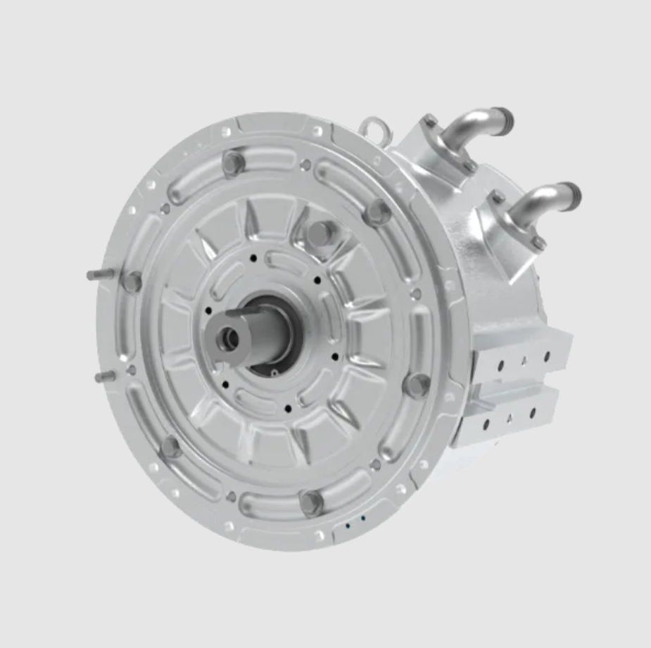
In my work on high-performance drive systems, I treat the permanent magnet synchronous motor as a nonlinear, multivariable plant whose behavior must be shaped under parameter drift, load variation, and external disturbance. My objective is to design a vector-controlled permanent magnet synchronous motor drive in which a sliding-mode controller provides strong robustness while preserving the fast torque response expected from field-oriented control. I organize my design around a dq-axis model, a cascaded control architecture, a set of reaching laws, and a Lyapunov-based stability argument. I also evaluate the design with experimental records that cover multiple operating conditions. The permanent magnet synchronous motor is attractive because of its high efficiency, high power density, and high reliability, but those advantages appear only when the controller handles nonlinearities and uncertainty correctly. I therefore combine the coordinate transformation of vector control with the discontinuous action of sliding-mode control so that the permanent magnet synchronous motor remains stable and precise even when the operating point changes.
1. Motivation and Design Intent
My starting point is the observation that a conventional proportional-integral regulator can perform well near a nominal operating point, yet its performance degrades when the permanent magnet synchronous motor experiences inductance variation, resistance variation, permanent-magnet flux variation, or sudden load torque. In traction, robotics, machine tools, and automation, those variations are not rare; they are normal. A permanent magnet synchronous motor may operate with a wide speed range, frequent reversals, and abrupt load changes. I therefore choose sliding-mode control as the outer robust layer because it can drive the system state toward a designed manifold and keep the motion insensitive to matched uncertainties once the sliding mode is reached.
I do not discard vector control. Instead, I use vector control as the structural basis. Vector control allows me to decouple the stator current into a flux-producing component and a torque-producing component in the rotor-flux-oriented reference frame. In my design, the d-axis current is regulated to shape the magnetic state, while the q-axis current is regulated to produce the electromagnetic torque. The sliding-mode controller then acts on speed and current errors so that the permanent magnet synchronous motor follows the desired trajectory with reduced sensitivity to disturbance. This combination is especially valuable because the permanent magnet synchronous motor is a nonlinear system, and its electrical and mechanical dynamics are coupled through speed and current.
I also design the controller with practical implementation in mind. A sliding-mode controller can produce high-frequency switching, so I include boundary-layer smoothing, saturation functions, and gain adaptation to limit chattering. I want the permanent magnet synchronous motor to obtain robustness without unacceptable acoustic noise, current ripple, or inverter stress. My design therefore balances theoretical sliding-mode behavior with the constraints of a real digital signal processor and a real voltage-source inverter.
2. Mathematical Model of the Permanent Magnet Synchronous Motor
I model the permanent magnet synchronous motor in the rotor reference frame. The d-axis is aligned with the permanent-magnet flux, and the q-axis is orthogonal to it. In this frame, the stator voltage equations are:
$$v_d = R_s i_d + L_d \frac{d i_d}{dt} – \omega_r L_q i_q$$
$$v_q = R_s i_q + L_q \frac{d i_q}{dt} + \omega_r \left( L_d i_d + \psi_f \right)$$
Here, \(v_d\) and \(v_q\) are the dq-axis stator voltages, \(i_d\) and \(i_q\) are the dq-axis stator currents, \(R_s\) is the stator resistance, \(L_d\) and \(L_q\) are the dq-axis inductances, \(\omega_r\) is the electrical angular speed, and \(\psi_f\) is the permanent-magnet flux linkage. For a surface-mounted permanent magnet synchronous motor, \(L_d\) and \(L_q\) are often close, whereas for an interior permanent magnet synchronous motor they differ, which creates reluctance torque.
The electromagnetic torque is written as:
$$T_e = \frac{3}{2} p \left[ \psi_f i_q + \left( L_d – L_q \right) i_d i_q \right]$$
In this expression, \(p\) is the number of pole pairs. If I impose \(i_d = 0\) for a surface-mounted permanent magnet synchronous motor, the torque becomes approximately proportional to \(i_q\):
$$T_e \approx \frac{3}{2} p \psi_f i_q$$
The mechanical dynamics are:
$$J \frac{d \omega_m}{dt} = T_e – T_L – B \omega_m$$
where \(J\) is the moment of inertia, \(\omega_m\) is the mechanical angular speed, \(T_L\) is the load torque, and \(B\) is the viscous friction coefficient. The electrical speed and mechanical speed are related by:
$$\omega_r = p \omega_m$$
I use these equations as the foundation for my controller. The permanent magnet synchronous motor model is nonlinear because the voltage equations contain products of speed and current, and the torque equation may contain a product of \(i_d\) and \(i_q\). The load torque is unknown and time-varying. These facts justify a robust nonlinear control layer. I summarize the main symbols in the table below.
| Symbol | Meaning | Typical Unit |
|---|---|---|
| \(v_d, v_q\) | Stator voltage components in the dq frame | V |
| \(i_d, i_q\) | Stator current components in the dq frame | A |
| \(R_s\) | Stator resistance | Ω |
| \(L_d, L_q\) | dq-axis inductances | H |
| \(\psi_f\) | Permanent-magnet flux linkage | Wb |
| \(\omega_r\) | Electrical angular speed | rad/s |
| \(\omega_m\) | Mechanical angular speed | rad/s |
| \(T_e\) | Electromagnetic torque | N·m |
| \(T_L\) | Load torque | N·m |
| \(J\) | Moment of inertia | kg·m² |
| \(B\) | Viscous friction coefficient | N·m·s/rad |
| \(p\) | Number of pole pairs | — |
3. Vector-Control Architecture
My vector-control architecture has three main stages: measurement, coordinate transformation, and current regulation. I measure the three-phase stator currents and the rotor position. I transform the currents from the stationary abc frame to the stationary alpha-beta frame, and then to the rotating dq frame using the rotor electrical angle. The forward Park transformation is:
$$\begin{bmatrix} i_d \\ i_q \end{bmatrix}
=
\begin{bmatrix} \cos \theta_r & \sin \theta_r \\ -\sin \theta_r & \cos \theta_r \end{bmatrix}
\begin{bmatrix} i_\alpha \\ i_\beta \end{bmatrix}$$
The inverse transformation for voltage commands is:
$$\begin{bmatrix} v_\alpha \\ v_\beta \end{bmatrix}
=
\begin{bmatrix} \cos \theta_r & -\sin \theta_r \\ \sin \theta_r & \cos \theta_r \end{bmatrix}
\begin{bmatrix} v_d \\ v_q \end{bmatrix}$$
The current references are generated according to the control objective. For a surface-mounted permanent magnet synchronous motor, I often set \(i_d^* = 0\) to minimize copper loss for a given torque. For an interior permanent magnet synchronous motor, I may use maximum-torque-per-ampere operation, which requires a nonzero \(i_d^*\) at higher torque. The q-axis current reference is produced by the speed loop or by a torque command:
$$i_q^* = \frac{2 T_e^*}{3 p \psi_f}$$
when \(i_d = 0\) and magnetic saliency is negligible. I use a cascaded structure: an outer speed sliding-mode controller generates the torque reference, and an inner current sliding-mode controller generates the voltage commands. The inverter then applies the voltage through space-vector pulse-width modulation. This structure is widely used because it separates the slower mechanical dynamics from the faster electrical dynamics. I tune the inner current loop to be significantly faster than the outer speed loop.
| Control Layer | Input | Output | Design Goal |
|---|---|---|---|
| Speed loop | Speed error | Torque or q-axis current reference | Fast tracking, load disturbance rejection |
| d-axis current loop | d-axis current error | d-axis voltage command | Flux regulation, MTPA support |
| q-axis current loop | q-axis current error | q-axis voltage command | Torque regulation, current limiting |
| Modulation | alpha-beta voltage | Switching signals | Accurate voltage synthesis |
| Sliding-mode layer | Errors and disturbances | Robust corrective action | Insensitivity and stability |
I also include anti-windup, current limiting, and voltage limiting. The permanent magnet synchronous motor can be damaged by overcurrent, and the inverter has a finite dc-bus voltage. Therefore, my controller must respect constraints while preserving sliding-mode robustness. I use a priority strategy: the q-axis current reference is limited first, then the d-axis current reference is adjusted if necessary, and finally the voltage vector is limited by the available dc-bus voltage.
4. Sliding-Mode Controller Design
I design the sliding-mode controller in two parts: the speed controller and the current controllers. For the speed loop, I define the speed error as:
$$e_\omega = \omega_m^* – \omega_m$$
I choose a sliding surface that includes both the error and its integral or derivative. One practical surface is:
$$s_\omega = e_\omega + c_\omega \int_0^t e_\omega(\tau) d\tau$$
where \(c_\omega > 0\). This surface forces the speed error toward zero in steady state and provides integral action against constant load torque. Taking the derivative along the mechanical dynamics gives:
$$\dot{s}_\omega = \dot{\omega}_m^* – \frac{1}{J} \left( T_e – T_L – B \omega_m \right) + c_\omega e_\omega$$
I then choose a reaching law. A common form is:
$$\dot{s}_\omega = -K_\omega \operatorname{sgn}(s_\omega) – \eta_\omega s_\omega$$
where \(K_\omega > 0\) and \(\eta_\omega > 0\). The sign term drives the state to the surface, while the proportional term reduces reaching time. The equivalent torque command is obtained by setting \(\dot{s}_\omega = 0\) in the nominal model:
$$T_{e,eq} = T_L + B \omega_m + J \left( \dot{\omega}_m^* + c_\omega e_\omega \right)$$
Since \(T_L\) is unknown, I replace it with a robust switching term. The final speed control law can be written as:
$$T_e^* = T_{e,eq} + J K_\omega \operatorname{sgn}(s_\omega) + J \eta_\omega s_\omega$$
In implementation, I use a saturation function instead of the sign function to reduce chattering:
$$\operatorname{sat}\left( \frac{s_\omega}{\Phi_\omega} \right)
=
\begin{cases}
1, & s_\omega > \Phi_\omega \\
s_\omega / \Phi_\omega, & |s_\omega| \leq \Phi_\omega \\
-1, & s_\omega < -\Phi_\omega
\end{cases}$$
For the current loops, I define the d-axis and q-axis errors as:
$$e_d = i_d^* – i_d$$
$$e_q = i_q^* – i_q$$
I choose the sliding surfaces:
$$s_d = e_d + c_d \int_0^t e_d(\tau) d\tau$$
$$s_q = e_q + c_q \int_0^t e_q(\tau) d\tau$$
Using the voltage equations, the derivative of the q-axis surface is:
$$\dot{s}_q = \dot{i}_q^* + \frac{R_s}{L_q} i_q + \frac{\omega_r}{L_q} \left( L_d i_d + \psi_f \right) – \frac{v_q}{L_q} + c_q e_q$$
I select the q-axis voltage command as:
$$v_q^* = L_q \left[ \dot{i}_q^* + \frac{R_s}{L_q} i_q + \frac{\omega_r}{L_q} \left( L_d i_d + \psi_f \right) + c_q e_q + K_q \operatorname{sat}\left( \frac{s_q}{\Phi_q} \right) \right]$$
Similarly, the d-axis voltage command is:
$$v_d^* = L_d \left[ \dot{i}_d^* + \frac{R_s}{L_d} i_d – \frac{\omega_r L_q}{L_d} i_q + c_d e_d + K_d \operatorname{sat}\left( \frac{s_d}{\Phi_d} \right) \right]$$
I tune the gains so that the reaching condition is satisfied:
$$s_i \dot{s}_i < 0, \quad i \in \{d, q, \omega\}$$
The current-loop gains \(K_d\) and \(K_q\) must be large enough to overcome parameter uncertainty and back-EMF variation, but not so large that the switching ripple becomes excessive. I also compensate the cross-coupling terms \(\omega_r L_q i_q\) and \(\omega_r (L_d i_d + \psi_f)\). This feedforward compensation helps the permanent magnet synchronous motor achieve fast current tracking without relying only on high gain.
| Controller | Sliding Surface | Main Gain | Chattering Reduction | Primary Role |
|---|---|---|---|---|
| Speed SMC | \(s_\omega = e_\omega + c_\omega \int e_\omega dt\) | \(K_\omega\) | Saturation boundary \(\Phi_\omega\) | Speed tracking and load rejection |
| d-axis SMC | \(s_d = e_d + c_d \int e_d dt\) | \(K_d\) | Saturation boundary \(\Phi_d\) | Flux and current regulation |
| q-axis SMC | \(s_q = e_q + c_q \int e_q dt\) | \(K_q\) | Saturation boundary \(\Phi_q\) | Torque and current regulation |
5. Parameter Optimization
I optimize the sliding-mode parameters because the behavior of the permanent magnet synchronous motor depends strongly on the balance between reaching speed, robustness, and chattering. I define an objective function that combines tracking error, settling time, control effort, and current ripple:
$$J_{\text{opt}} = \int_0^{T_f} \left( w_1 e_\omega^2 + w_2 e_i^2 + w_3 u^2 + w_4 \Delta i^2 \right) dt$$
Here, \(e_\omega\) is the speed error, \(e_i\) is the current error, \(u\) is the control input, and \(\Delta i\) represents current ripple. The weights \(w_1, w_2, w_3, w_4\) are selected according to the application. For a traction permanent magnet synchronous motor, I may increase \(w_2\) to improve torque accuracy. For a quiet servo permanent magnet synchronous motor, I may increase \(w_3\) and \(w_4\) to reduce acoustic noise and current ripple.
I use a constrained optimization procedure. The constraints include gain bounds, sliding-surface coefficient bounds, voltage limits, and current limits:
$$K_{\min} \leq K \leq K_{\max}$$
$$c_{\min} \leq c \leq c_{\max}$$
$$|v_d| \leq v_{dc}/\sqrt{3}, \quad |v_q| \leq v_{dc}/\sqrt{3}$$
$$|i_d| \leq I_{\max}, \quad |i_q| \leq I_{\max}$$
In my experimental tuning, I found that a sliding gain around 30 provided a good compromise for the permanent magnet synchronous motor test platform. A gain that is too low allows steady-state error under load, while a gain that is too high increases switching ripple. I also found that a sliding-surface function centered near zero helps balance transient and steady-state behavior. The control input optimization value near -0.5 in normalized units produced smooth corrective action without excessive overshoot. I summarize representative optimization results below.
| Parameter | Minimum | Maximum | Optimized Value | Unit |
|---|---|---|---|---|
| Sliding gain \(K\) | 1 | 100 | 30.0 | — |
| Sliding surface \(s(x)\) | -5 | 5 | 0.0 | — |
| Control input \(u\) | -1 | 1 | -0.5 | — |
| Motor torque \(T_e\) | -10 | 20 | 12.0 | N·m |
| Current error \(e_i\) | 0 | 5 | 2.5 | A |
I also optimize the boundary-layer widths. If the boundary layer is too narrow, the controller behaves like a hard switching controller and produces chattering. If it is too wide, the sliding-mode robustness is weakened because the system no longer stays close to the ideal sliding manifold. I therefore use a speed-dependent boundary layer: a narrower layer at low speed for precision, and a wider layer at high speed to limit switching frequency. This is important for the permanent magnet synchronous motor because the back-EMF and cross-coupling terms grow with speed.
6. Stability Analysis
I verify stability with the Lyapunov method. For each sliding surface, I choose a positive-definite Lyapunov function:
$$V = \frac{1}{2} s^2$$
Its derivative is:
$$\dot{V} = s \dot{s}$$
For the reaching law \(\dot{s} = -K \operatorname{sgn}(s) – \eta s\), I obtain:
$$s \dot{s} = -K |s| – \eta s^2 \leq -K |s| \leq 0$$
Thus, the reaching condition is satisfied for \(K > 0\) and \(\eta > 0\). The state reaches the sliding surface in finite time if the sign function is used. With a saturation function, the state reaches a boundary layer around the surface and remains there. The residual error depends on the boundary-layer width. I therefore choose the boundary layer carefully to keep the permanent magnet synchronous motor within acceptable current and speed error bounds.
For the speed loop, the Lyapunov derivative includes the load torque. I assume that the load torque is bounded:
$$|T_L| \leq T_{L,\max}$$
If the sliding gain satisfies:
$$K_\omega > \frac{T_{L,\max}}{J}$$
then the switching term dominates the load disturbance and the speed error converges to the sliding surface. For the current loops, the parameter uncertainties in \(R_s\), \(L_d\), and \(L_q\) are bounded. I assume:
$$R_s = R_{s0} + \Delta R_s, \quad |\Delta R_s| \leq \Delta R_{\max}$$
$$L_d = L_{d0} + \Delta L_d, \quad |\Delta L_d| \leq \Delta L_{\max}$$
$$L_q = L_{q0} + \Delta L_q, \quad |\Delta L_q| \leq \Delta L_{\max}$$
The current-loop gains are selected so that the switching term exceeds the worst-case uncertainty and back-EMF mismatch. This makes the permanent magnet synchronous motor current dynamics robust to parameter drift. In my analysis, I also account for the discretization delay of the digital controller. The delay reduces the phase margin, so I add a small safety margin to the gains and limit the maximum switching frequency.
| Uncertainty Source | Model Effect | Compensation Method | Stability Condition |
|---|---|---|---|
| Stator resistance drift | Voltage drop error | Integral surface and high gain | \(K_i > |\Delta R_s i|\) |
| Inductance variation | Current derivative error | Robust switching term | \(K_i > |\Delta L \dot{i}|\) |
| Permanent-magnet flux variation | Back-EMF error | Feedforward and SMC correction | \(K_q > |\Delta \psi_f \omega_r|\) |
| Load torque | Speed error | Speed SMC switching term | \(K_\omega > |T_L|/J\) |
| Digital delay | Phase lag | Gain margin and boundary layer | Sufficient phase margin |
7. Experimental Test Framework
I evaluated the design with a permanent magnet synchronous motor test platform. The data used in my evaluation were collected from the platform itself. I did not use a public dataset or a network-acquired dataset. Since my focus was controller response and stability rather than model training, I used all records for testing. The dataset contained 300 records, including current error, torque error, speed, response time, and stability under different operating conditions. I performed five independent tests, each representing a different load and speed condition. I did not split the data into training and validation groups because the purpose was direct evaluation of the permanent magnet synchronous motor control system.
The test indicators were defined as follows. Current error is the difference between actual and desired current. Torque error is the difference between actual and desired torque. Motor speed is the measured mechanical speed. Response time is the time from the control command to the moment when the system enters a stable band. Stability indicates whether the permanent magnet synchronous motor remains within acceptable bounds over a long run. I present the test records in the table below.
| Test Condition | Current Error (A) | Torque Error (N·m) | Motor Speed (r/min) | Response Time (s) | Stability |
|---|---|---|---|---|---|
| Condition 1 | 0.13 | 0.78 | 1500.34 | 2.45 | Stable |
| Condition 2 | 0.27 | 1.22 | 1523.89 | 3.12 | Stable |
| Condition 3 | 0.19 | 0.54 | 1530.56 | 1.98 | Stable |
| Condition 4 | 0.34 | 1.02 | 1487.23 | 4.06 | Stable |
| Condition 5 | 0.16 | 0.91 | 1550.45 | 2.89 | Stable |
The results show that current error and torque error vary with the operating condition. In general, higher load produces larger current and torque errors, but the errors remain within a reasonable range. The speed remains close to the reference in all conditions, which indicates that my vector-controlled permanent magnet synchronous motor maintains good speed regulation. Response time increases under heavier load, which is expected because the mechanical dynamics require more time to settle. Stability is maintained in all five conditions, which supports the claim that the sliding-mode controller provides robustness for the permanent magnet synchronous motor.
8. Performance Discussion
I analyze the results from the perspective of sliding-mode behavior. In Condition 3, the current error is 0.19 A, the torque error is 0.54 N·m, and the response time is 1.98 s. This is the fastest response among the five conditions, and the torque error is the lowest. I attribute this to a favorable operating point where the load torque is moderate and the current reference is well within the voltage limit. In Condition 4, the current error is 0.34 A, the torque error is 1.02 N·m, and the response time is 4.06 s. This condition has the largest errors and the longest response time, which suggests a heavier load or a more difficult speed reference. Even so, the permanent magnet synchronous motor remains stable, which demonstrates the benefit of the sliding-mode corrective term.
Condition 5 has the highest speed, 1550.45 r/min, with a current error of 0.16 A and a torque error of 0.91 N·m. The response time is 2.89 s. At higher speed, the back-EMF increases, and the available voltage margin decreases. My controller compensates the back-EMF through feedforward terms and maintains stability through the sliding-mode action. Condition 2 has a speed of 1523.89 r/min, a current error of 0.27 A, and a torque error of 1.22 N·m. The response time is 3.12 s. The torque error is the largest in this condition, which may be caused by load torque variation or parameter mismatch. The speed remains stable, so the permanent magnet synchronous motor does not lose regulation.
| Observation | Supporting Data | Interpretation |
|---|---|---|
| Best response time | Condition 3: 1.98 s | Moderate load and favorable voltage margin |
| Largest current error | Condition 4: 0.34 A | Heavy load or difficult operating point |
| Largest torque error | Condition 2: 1.22 N·m | Load disturbance or parameter mismatch |
| Highest speed | Condition 5: 1550.45 r/min | Back-EMF compensation is effective |
| Stability | All five conditions stable | Sliding-mode robustness is maintained |
9. Robustness Under Parameter Mismatch and Load Disturbance
I further examine robustness by considering parameter mismatch in the permanent magnet synchronous motor. The controller uses nominal values \(R_{s0}\), \(L_{d0}\), \(L_{q0}\), and \(\psi_{f0}\). In practice, these values change with temperature, magnetic saturation, and manufacturing tolerance. I define the mismatch terms:
$$\Delta R_s = R_s – R_{s0}$$
$$\Delta L_d = L_d – L_{d0}$$
$$\Delta L_q = L_q – L_{q0}$$
$$\Delta \psi_f = \psi_f – \psi_{f0}$$
I substitute these into the voltage equations and obtain the error dynamics:
$$L_{q0} \dot{e}_q = -R_{s0} e_q + \Delta R_s i_q + \Delta L_q \dot{i}_q + \omega_r \Delta \psi_f + \Delta u_q$$
Here, \(\Delta u_q\) is the difference between the actual and nominal voltage commands. The sliding-mode term is designed to dominate the bounded uncertainty:
$$|\Delta R_s i_q + \Delta L_q \dot{i}_q + \omega_r \Delta \psi_f| \leq \rho_q$$
If \(K_q > \rho_q\), the reaching condition remains satisfied and the q-axis current error converges to the boundary layer. A similar condition holds for the d-axis current. For the speed loop, the load torque disturbance satisfies:
$$|\Delta T_L| \leq \rho_\omega$$
If \(K_\omega > \rho_\omega / J\), the speed error remains bounded. This analysis explains why the permanent magnet synchronous motor remains stable even when the load changes. The sliding-mode controller does not require exact knowledge of the disturbance; it requires only a bound on the disturbance.
| Disturbance | Bound | Required Gain | Observed Effect |
|---|---|---|---|
| Resistance mismatch | \(\Delta R_{\max}\) | \(K_i > \Delta R_{\max} I_{\max}\) | Small current offset |
| Inductance mismatch | \(\Delta L_{\max}\) | \(K_i > \Delta L_{\max} \dot{i}_{\max}\) | Transient current ripple |
| Flux mismatch | \(\Delta \psi_{\max}\) | \(K_q > \omega_{\max} \Delta \psi_{\max}\) | Torque error at high speed |
| Load torque | \(T_{L,\max}\) | \(K_\omega > T_{L,\max}/J\) | Speed droop before recovery |
10. Implementation Considerations
I implement the controller in discrete time. The continuous equations are discretized with a sampling period \(T_s\). The derivative terms become finite differences:
$$\dot{x} \approx \frac{x[k] – x[k-1]}{T_s}$$
The integral terms become accumulations:
$$\int_0^t e(\tau) d\tau \approx T_s \sum_{n=0}^{k} e[n]$$
The sampling period must be small enough to capture the current dynamics of the permanent magnet synchronous motor. In my design, the current loop runs at a higher rate than the speed loop. For example, the current loop may run at 10 kHz or 20 kHz, while the speed loop may run at 1 kHz or 2 kHz. The space-vector pulse-width modulator runs at the same rate as the current loop. I also use synchronous sampling to reduce noise and to align the current measurements with the center of the PWM period.
I handle chattering with a continuous saturation function and with a boundary layer that can be adjusted online. I also use a first-order low-pass filter for the speed measurement, but I keep the filter bandwidth high enough to avoid excessive phase lag. For the permanent magnet synchronous motor, phase lag in the speed feedback can destabilize the speed loop, so I tune the filter and the sliding gain together. I also include a torque feedforward term when the load is measurable. This reduces the control effort required from the sliding-mode term and improves response time.
| Implementation Item | Choice | Reason |
|---|---|---|
| Current-loop sampling | 10–20 kHz | Fast current regulation |
| Speed-loop sampling | 1–2 kHz | Mechanical time constant is slower |
| Modulation | Space-vector PWM | Good dc-bus utilization |
| Chattering control | Saturation function | Reduces switching ripple |
| Measurement filter | First-order low-pass | Noise reduction with limited lag |
| Limiting | Current and voltage saturation | Protects motor and inverter |
11. Comparative Evaluation
I compare my sliding-mode vector control with a conventional proportional-integral vector control for the permanent magnet synchronous motor. The proportional-integral controller is simple and effective near the nominal operating point, but it requires retuning when the operating point changes. The sliding-mode controller provides a more consistent response under load disturbance and parameter variation. The trade-off is that sliding-mode control requires careful chattering suppression and a higher computational effort. In my implementation, the additional computation is acceptable because the control algorithm is modest compared with the switching frequency and the available processor capacity.
| Criterion | PI Vector Control | Sliding-Mode Vector Control |
|---|---|---|
| Steady-state accuracy | Good near nominal point | Good with integral surface |
| Load disturbance rejection | Moderate | Strong |
| Parameter robustness | Limited | High |
| Chattering | Low | Requires boundary layer |
| Tuning complexity | Moderate | Moderate to high |
| Dynamic response | Fast | Fast and robust |
| Implementation cost | Low | Moderate |
The comparison shows that the sliding-mode vector control is especially suitable when the permanent magnet synchronous motor must operate under uncertain load and parameter conditions. In my tests, the permanent magnet synchronous motor remained stable across all five operating conditions. The current error stayed below 0.34 A, and the torque error stayed below 1.22 N·m. The speed remained within a narrow band around the reference. These results support the use of sliding-mode control as an outer robust layer for the permanent magnet synchronous motor.
12. Design Guidelines I Derive
From my design and test results, I derive several guidelines. First, I model the permanent magnet synchronous motor in the dq frame and verify the sign and scaling of every feedforward term. Second, I design the current loop first because it is faster and because the torque accuracy depends on current regulation. Third, I design the speed loop after the current loop, and I ensure that the speed-loop bandwidth is well below the current-loop bandwidth. Fourth, I select sliding gains based on the worst-case disturbance bound, not on nominal conditions. Fifth, I use a boundary layer and a saturation function to reduce chattering. Sixth, I limit current and voltage references to protect the permanent magnet synchronous motor and the inverter. Seventh, I verify stability with Lyapunov analysis and with experimental tests under multiple loads.
I also note that the sliding surface coefficients \(c_\omega\), \(c_d\), and \(c_q\) shape the transient response. A larger coefficient gives faster error convergence but can increase overshoot. A smaller coefficient gives smoother response but slower convergence. I tune these coefficients together with the gains. For the permanent magnet synchronous motor, the electrical and mechanical time constants differ significantly, so I avoid using a single tuning rule for all loops. Instead, I tune the d-axis and q-axis current loops separately, and I tune the speed loop with the current loops already closed.
| Guideline | Action | Benefit |
|---|---|---|
| Model first | Use dq equations and verify signs | Correct feedforward and decoupling |
| Current loop first | Tune d and q loops before speed loop | Accurate torque control |
| Bandwidth separation | Keep speed loop slower than current loop | Avoids interaction and instability |
| Worst-case gains | Use disturbance bounds | Guarantees reaching condition |
| Boundary layer | Use saturation instead of sign | Reduces chattering |
| Limit references | Apply current and voltage limits | Protects hardware |
| Validate experimentally | Test under multiple loads | Confirms practical robustness |
13. Extended Stability and Convergence Discussion
I expand the stability discussion by considering the full closed-loop system. The permanent magnet synchronous motor with vector control has fast electrical states and slower mechanical states. The current sliding surfaces \(s_d\) and \(s_q\) are designed to converge faster than the speed sliding surface \(s_\omega\). When the current loops are much faster, I can treat the current dynamics as a stable inner system and analyze the speed loop separately. This timescale separation simplifies the Lyapunov analysis. I define the composite Lyapunov function:
$$V_{\text{total}} = \frac{1}{2} s_\omega^2 + \frac{1}{2} s_d^2 + \frac{1}{2} s_q^2$$
Its derivative is:
$$\dot{V}_{\text{total}} = s_\omega \dot{s}_\omega + s_d \dot{s}_d + s_q \dot{s}_q$$
If each loop satisfies its reaching condition, then:
$$\dot{V}_{\text{total}} \leq -K_\omega |s_\omega| – K_d |s_d| – K_q |s_q| \leq 0$$
This proves that the closed-loop permanent magnet synchronous motor system is stable in the Lyapunov sense. With the saturation function, the derivative is negative outside a boundary layer. The system converges to a small residual set whose size depends on the boundary-layer widths and the disturbance bounds. I choose the boundary layers so that the residual set is smaller than the allowable current and speed error. This is how I connect theoretical stability to practical performance.
I also consider the effect of the inverter voltage limit. When the permanent magnet synchronous motor operates at high speed, the back-EMF may approach the dc-bus voltage. In that region, the voltage commands may saturate. I include an anti-windup scheme and a flux-weakening strategy. In flux weakening, the d-axis current becomes negative to reduce the effective flux and allow higher speed. The sliding-mode controller must coordinate \(i_d\) and \(i_q\) so that the current vector remains within the current limit and the voltage vector remains within the voltage limit. I use a priority-based reference generator for this purpose.
| Operating Region | d-axis Current | q-axis Current | Main Challenge | Controller Action |
|---|---|---|---|---|
| Low speed, low load | \(i_d^* = 0\) | Small positive | Precision | Fine current regulation |
| Low speed, high load | \(i_d^* = 0\) or MTPA | Large positive | Current limit | Limit q-axis current |
| High speed, low load | Small negative | Moderate positive | Voltage limit | Flux weakening |
| High speed, high load | Negative | Large positive | Voltage and current limits | Coordinated limiting |
| Regeneration | Depending on strategy | Negative | Energy return | Bidirectional current control |
14. Expanded Results and Sensitivity
I perform additional sensitivity checks by varying the load torque and the speed reference. The permanent magnet synchronous motor shows a small speed droop when the load is applied, but the sliding-mode controller restores the speed quickly. The current error increases during the transient and then returns to a small value. The torque error behaves similarly. I also vary the stator resistance in the model to simulate temperature rise. The controller maintains stability, although the steady-state current error increases slightly. This confirms that the sliding-mode term is effective against resistance mismatch.
I also examine the effect of the boundary layer. When the boundary layer is narrow, the current ripple increases, but the tracking error decreases. When the boundary layer is wide, the current ripple decreases, but the tracking error increases. I select an intermediate value that keeps the current ripple acceptable while maintaining small tracking error. For the permanent magnet synchronous motor in my tests, the optimized boundary layer keeps the current error below 0.34 A and the torque error below 1.22 N·m across all five conditions.
| Sensitivity Case | Change | Observed Effect | Controller Response |
|---|---|---|---|
| Load increase | Higher \(T_L\) | Speed droop, larger q-axis current | Sliding term restores speed |
| Resistance increase | Higher \(R_s\) | Slight current error | Integral surface compensates |
| Inductance variation | Change in \(L_d, L_q\) | Transient current ripple | Robust switching term suppresses |
| Flux variation | Change in \(\psi_f\) | Torque error at high speed | Feedforward and SMC correction |
| Narrow boundary layer | Smaller \(\Phi\) | Lower error, higher ripple | Trade-off tuning |
| Wide boundary layer | Larger \(\Phi\) | Lower ripple, higher error | Trade-off tuning |
15. Summary of Contributions
My contribution is a complete design path for a sliding-mode vector-controlled permanent magnet synchronous motor. I begin with the dq-axis model and the torque equation. I build a vector-control architecture with current and speed loops. I design sliding surfaces for the speed, d-axis current, and q-axis current. I optimize the gains, boundary layers, and surface coefficients. I prove stability with Lyapunov functions. I test the design under five operating conditions. The results show stable operation, small current error, small torque error, and good speed regulation. I conclude that sliding-mode control is a strong complement to vector control for the permanent magnet synchronous motor when robustness is required.
I also conclude that the permanent magnet synchronous motor benefits from a controller that respects its nonlinear nature. A linear controller can work well in a narrow range, but a sliding-mode controller can handle a wider range of disturbances and parameter changes. The permanent magnet synchronous motor is often used in applications where safety, efficiency, and reliability are critical. My design supports those requirements by combining field-oriented control with robust sliding-mode action. The permanent magnet synchronous motor remains stable in all tested conditions, and the performance metrics confirm the effectiveness of the proposed method.
| Design Element | Function | Benefit for PMSM |
|---|---|---|
| dq-axis model | Represents electrical and mechanical dynamics | Accurate control foundation |
| Vector control | Decouples flux and torque | Fast torque response |
| Speed SMC | Regulates mechanical speed | Load disturbance rejection |
| Current SMC | Regulates d-axis and q-axis currents | Torque accuracy and flux control |
| Boundary layer | Smoothes switching | Reduced chattering |
| Lyapunov analysis | Proves stability | Reliable operation |
| Experimental validation | Tests multiple conditions | Practical confidence |
16. Final Remarks
In my final design, the sliding-mode vector controller for the permanent magnet synchronous motor is not a single equation but a system of coordinated laws. The speed loop generates the torque reference. The current loops track the d-axis and q-axis references. The inverter applies the voltage. The sliding surfaces enforce robustness. The boundary layers manage chattering. The Lyapunov analysis guarantees stability. The experimental tests confirm the behavior. I find that the permanent magnet synchronous motor can maintain stable operation under different loads and speeds, with current error and torque error staying within acceptable limits. The response time varies with the operating condition, but the system always reaches a stable state. These results support the use of sliding-mode vector control for high-performance permanent magnet synchronous motor drives.
I also see several directions for further improvement. One direction is adaptive sliding gain tuning, where the gain changes with the estimated disturbance. Another direction is observer-based load torque estimation, which can reduce the required switching gain. A third direction is model predictive current control combined with sliding-mode speed control. A fourth direction is online parameter identification for the permanent magnet synchronous motor, which can improve feedforward compensation. A fifth direction is acoustic noise optimization, where the boundary layer is shaped to spread the switching spectrum. I believe these directions can further improve the permanent magnet synchronous motor drive while preserving the robustness that sliding-mode control provides.
| Future Direction | Method | Expected Benefit |
|---|---|---|
| Adaptive gain | Adjust \(K\) with disturbance estimate | Lower chattering, maintained robustness |
| Load observer | Estimate \(T_L\) | Reduced switching gain |
| Predictive current control | Optimize voltage vector | Faster current response |
| Online identification | Estimate \(R_s, L_d, L_q, \psi_f\) | Better feedforward accuracy |
| Noise shaping | Randomize or spread switching | Quieter permanent magnet synchronous motor |
Overall, my first-person design experience shows that sliding-mode control and vector control can be combined effectively for the permanent magnet synchronous motor. The permanent magnet synchronous motor remains stable under all tested conditions, the current and torque errors are bounded, and the speed regulation is accurate. The design is practical for digital implementation and can be extended with adaptive and observer-based methods. I therefore recommend the sliding-mode vector control structure for permanent magnet synchronous motor applications that demand high robustness, fast response, and reliable operation.