
I approach the analysis of electric vehicle traction systems from the viewpoint of an electric drive engineer who needs to connect electromagnetic design, power electronics, real-time control, and vehicle-level energy management. The permanent magnet synchronous motor is one of the most important actuators in this chain because it offers high efficiency, high power density, fast torque response, and a wide speed range when it is paired with an appropriate inverter and control strategy. In my assessment, the permanent magnet synchronous motor is not simply a component choice; it is a system-level decision that affects acceleration feel, gradeability, cruising efficiency, thermal safety, acoustic comfort, and the overall architecture of the electric drive unit. The permanent magnet synchronous motor therefore deserves a control strategy that is layered, operating-region aware, and validated through integrated testing.
I organize my discussion around four connected layers. The first layer is the physical and electromagnetic behavior of the permanent magnet synchronous motor, including rotor construction and operating principles. The second layer is the drive system composition, where the permanent magnet synchronous motor interacts with the inverter, controller, sensors, and cooling circuit. The third layer is the core control architecture, especially field-oriented vector control and the decoupled current loops that make torque and flux controllable. The fourth layer is the operating-region strategy, where maximum torque per ampere control supports low-speed high-torque operation and flux weakening supports high-speed operation. I then connect these layers to an integrated electric drive case and compare performance indicators. Throughout this analysis, I use tables and formulas to make the relationships compact and repeatable.
Table 1. Classification and practical behavior of the permanent magnet synchronous motor.
| Feature | Interior permanent magnet synchronous motor | Surface-mounted permanent magnet synchronous motor |
|---|---|---|
| Magnet location | Magnets are buried inside the rotor core. | Magnets are attached to the rotor surface. |
| Reluctance torque | Strong because the d-axis and q-axis inductances differ. | Weak or nearly zero because the magnetic circuit is close to uniform. |
| Mechanical strength | High, which supports high-speed operation. | Lower, because magnets are exposed to centrifugal stress. |
| Air-gap flux waveform | Can be designed for acceptable sinusoidal quality with careful shaping. | Usually very sinusoidal and produces low torque ripple. |
| Field weakening capability | Good, because d-axis current can oppose the magnet flux. | More limited, because the effective air gap is larger. |
| Manufacturing cost | Higher due to magnet insertion, rotor lamination geometry, and tooling complexity. | Generally lower, but magnet retention still needs care. |
| Typical application | High-performance traction, wide-speed-range electric vehicles, and high-torque drive units. | Low-speed or cost-sensitive drives, auxiliary motors, and some compact traction units. |
When I compare the two structures, I do not treat one as universally superior. The interior permanent magnet synchronous motor is often preferred for traction because it can exploit reluctance torque and because its rotor structure tolerates high-speed operation. The surface-mounted permanent magnet synchronous motor is attractive when smooth torque and simple magnetic behavior are more important than wide-speed field weakening. For a vehicle, the selection depends on the mission profile. A city vehicle may spend most of its time in low-speed and medium-speed operation, while a highway-oriented vehicle needs efficient high-speed cruising and strong field weakening. A commercial vehicle may prioritize continuous torque and thermal robustness. These differences explain why control strategy must be matched to the permanent magnet synchronous motor structure and to the vehicle duty cycle.
The electromagnetic principle of the permanent magnet synchronous motor can be expressed through the synchronous speed relationship, the back electromotive force, and the electromagnetic torque. If the stator is supplied with a balanced three-phase current set, the stator produces a rotating magnetomotive force. The rotor permanent magnets produce a rotor flux. The interaction between the stator current and the rotor flux produces torque. The rotor speed is synchronized with the fundamental frequency of the stator current, which gives the following relationship:
$$ n_s = \frac{60 f}{p} $$
Here, \(n_s\) is the synchronous speed in revolutions per minute, \(f\) is the stator electrical frequency, and \(p\) is the number of pole pairs. I use this relationship as the first check in any control design because it links the inverter switching and modulation capability to the mechanical speed requirement. A high-speed permanent magnet synchronous motor needs a high fundamental frequency, and the controller sampling rate, current loop bandwidth, and inverter switching frequency must all support that frequency.
The back electromotive force of the permanent magnet synchronous motor is approximately proportional to speed and magnet flux:
$$ E = 4.44 f N \Phi k_w $$
In this expression, \(N\) is the number of turns per phase, \(\Phi\) is the flux per pole, and \(k_w\) is the winding factor. As speed rises, the back electromotive force rises. At some speed, the required terminal voltage approaches the maximum voltage that the inverter can deliver. This voltage limit is the origin of the base speed and the need for field weakening. The permanent magnet synchronous motor cannot reduce its magnet flux mechanically, so the controller must reduce the effective flux by injecting negative d-axis current. This is one of the central themes of my analysis.
The torque of the permanent magnet synchronous motor in the d-q reference frame is written as follows:
$$ T_e = \frac{3}{2} p \left[ \psi_f i_q + (L_d – L_q) i_d i_q \right] $$
Here, \(T_e\) is electromagnetic torque, \(\psi_f\) is the permanent magnet flux linkage, \(i_d\) and \(i_q\) are the d-axis and q-axis currents, and \(L_d\) and \(L_q\) are the d-axis and q-axis inductances. For a surface-mounted permanent magnet synchronous motor, \(L_d \approx L_q\), so the reluctance term is small and the torque is approximately proportional to \(i_q\). For an interior permanent magnet synchronous motor, \(L_d < L_q\), so a negative \(i_d\) can produce additional reluctance torque. This equation is the foundation of every operating-region strategy that follows.
Table 2. Performance advantages that I associate with the permanent magnet synchronous motor in electric vehicle traction.
| Performance dimension | Behavior of the permanent magnet synchronous motor | Practical consequence for the electric vehicle |
|---|---|---|
| Excitation loss | The rotor flux is provided by permanent magnets, so there is no separate excitation winding loss. | Higher efficiency in many operating points, especially under partial load. |
| Power density | High-energy permanent magnets allow a compact magnetic circuit. | Lower mass and volume for a given torque and power level. |
| Torque response | Current can be controlled quickly in the stator, and the rotor flux is always present. | Fast acceleration response and improved drivability. |
| Speed range | With field weakening, the permanent magnet synchronous motor can operate above base speed. | One motor can cover low-speed launch and high-speed cruising, reducing the need for multispeed gearing. |
| Control precision | Field-oriented control allows independent control of flux and torque current components. | Accurate speed and torque regulation over a wide operating range. |
| Thermal behavior | Rotor loss is low because the rotor does not carry excitation current. | Cooling can focus on stator copper loss and inverter losses, which simplifies thermal management. |
| Acoustic behavior | Torque ripple can be controlled through design and current waveform shaping. | Lower electromagnetic noise and a quieter cabin. |
The drive system of an electric vehicle is not only the permanent magnet synchronous motor. I see it as a tightly coupled assembly of the motor body, the power inverter, the controller, and the sensing network. The motor body includes the stator core, stator winding, rotor magnets, shaft, bearings, and cooling passages. The power inverter converts dc power from the battery into three-phase ac power. The controller executes the field-oriented algorithm, coordinate transformations, current regulation, speed regulation, field weakening logic, and protection functions. The sensors provide rotor position, phase currents, dc-link voltage, and temperature information. If any of these subsystems is poorly matched, the permanent magnet synchronous motor cannot reach its intended performance.
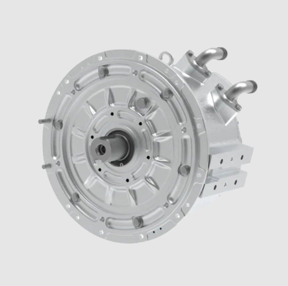
Table 3. Core components of a permanent magnet synchronous motor drive system and the parameters I monitor during design.
| Component | Core function | Key parameters |
|---|---|---|
| Permanent magnet synchronous motor body | Electromechanical energy conversion from electrical power to mechanical power. | Rated power 50 to 200 kW, rated torque 150 to 500 N·m, pole pairs, stator resistance, d-axis inductance, q-axis inductance, magnet flux linkage. |
| Power inverter | Converts dc battery voltage into controllable three-phase ac voltage and current. | Switching frequency 10 to 20 kHz, dc-link voltage, phase current rating, efficiency 98% to 99%, thermal resistance. |
| Controller | Executes vector control, field weakening, protection, and communication functions. | Main frequency around 300 MHz, current loop response below 1 ms, PWM resolution, ADC sampling synchronization. |
| Position sensor | Provides rotor electrical angle for Park transformation and field orientation. | Accuracy about ±0.1 electrical degree, resolution, offset error, delay compensation. |
| Current sensor | Measures phase or dc-link current for closed-loop current control and protection. | Measurement error below 1%, bandwidth, linearity, common-mode rejection. |
| Temperature sensor | Monitors stator winding, rotor, inverter, and coolant temperatures. | Thermal time constant, accuracy, placement, derating threshold. |
I consider vector control the backbone of permanent magnet synchronous motor traction control. The purpose of vector control is to transform the three-phase stationary variables into a rotating reference frame that moves with the rotor flux. In that frame, the permanent magnet synchronous motor behaves more like a separately excited dc machine from the control perspective: one current component controls flux and the other controls torque. This decoupling is what gives the permanent magnet synchronous motor fast and accurate torque response. Without it, the controller would struggle to separate magnet flux effects, reluctance effects, and speed-dependent voltage effects.
The first step in vector control is the Clarke transformation, which converts the three-phase stationary currents into two-phase stationary currents:
$$ \begin{bmatrix} i_\alpha \\ i_\beta \end{bmatrix} = \frac{2}{3} \begin{bmatrix} 1 & -\frac{1}{2} & -\frac{1}{2} \\ 0 & \frac{\sqrt{3}}{2} & -\frac{\sqrt{3}}{2} \end{bmatrix} \begin{bmatrix} i_a \\ i_b \\ i_c \end{bmatrix} $$
The second step is the Park transformation, which rotates the two-phase stationary frame into the d-q frame aligned with the rotor flux:
$$ \begin{bmatrix} i_d \\ i_q \end{bmatrix} = \begin{bmatrix} \cos\theta_e & \sin\theta_e \\ -\sin\theta_e & \cos\theta_e \end{bmatrix} \begin{bmatrix} i_\alpha \\ i_\beta \end{bmatrix} $$
Here, \(\theta_e\) is the electrical rotor angle. The inverse Park transformation is used to convert the desired d-axis and q-axis voltages back into the stationary frame before space-vector pulse-width modulation:
$$ \begin{bmatrix} v_\alpha \\ v_\beta \end{bmatrix} = \begin{bmatrix} \cos\theta_e & -\sin\theta_e \\ \sin\theta_e & \cos\theta_e \end{bmatrix} \begin{bmatrix} v_d \\ v_q \end{bmatrix} $$
In the d-q frame, the voltage equations of the permanent magnet synchronous motor are:
$$ v_d = R_s i_d + L_d \frac{d i_d}{d t} – \omega_e L_q i_q $$
$$ v_q = R_s i_q + L_q \frac{d i_q}{d t} + \omega_e (L_d i_d + \psi_f) $$
These equations show two important cross-coupling terms. The term \(-\omega_e L_q i_q\) appears in the d-axis voltage equation, and the term \(+\omega_e (L_d i_d + \psi_f)\) appears in the q-axis voltage equation. If I ignore these terms, the current loops will interact as speed rises. The d-axis current command will disturb the q-axis current, and the q-axis current command will disturb the d-axis current. The permanent magnet synchronous motor may still rotate, but the torque response will become sluggish, current tracking will degrade, and the controller may need excessive gains that amplify noise. Therefore, I always include feedforward decoupling in a high-performance permanent magnet synchronous motor controller.
A practical current loop with proportional-integral regulation and decoupling can be written as:
$$ v_d^* = G_{PI,d}(s)(i_d^* – i_d) – \omega_e L_q i_q $$
$$ v_q^* = G_{PI,q}(s)(i_q^* – i_q) + \omega_e (L_d i_d + \psi_f) $$
The proportional-integral controller is:
$$ G_{PI}(s) = K_p + \frac{K_i}{s} $$
I tune the d-axis and q-axis current loops according to the respective inductance values. The bandwidth of the current loop must be high enough to track fast torque commands, but not so high that switching noise, sampling delay, and dead-time effects dominate. In my experience, the current loop bandwidth is often set to one-tenth or less of the sampling frequency, with additional phase margin reserved for the computation delay and PWM update delay. The permanent magnet synchronous motor has a fast electrical time constant, so the controller must respect the digital delay:
$$ T_d \approx 1.5 T_s $$
Here, \(T_s\) is the sampling period. This delay appears in the closed-loop current transfer function and reduces phase margin. When I increase the switching frequency or the control sampling rate, I can push the current loop bandwidth higher, but this increases inverter losses. The design is therefore a trade-off between dynamic response and efficiency.
Table 4. Vector control modules and their functions for the permanent magnet synchronous motor.
| Module | Input | Output | Function |
|---|---|---|---|
| Clarke transformation | Three-phase currents \(i_a, i_b, i_c\) | Two-phase stationary currents \(i_\alpha, i_\beta\) | Reduces three-phase variables to an equivalent two-axis representation. |
| Park transformation | \(i_\alpha, i_\beta\) and rotor angle \(\theta_e\) | d-axis and q-axis currents \(i_d, i_q\) | Aligns current control with the rotor flux axis. |
| Current decoupling | \(i_d, i_q, \omega_e\) | Feedforward voltage terms | Compensates cross-coupling between d-axis and q-axis dynamics. |
| PI current regulators | Current errors \(i_d^* – i_d\) and \(i_q^* – i_q\) | Voltage commands \(v_d^*, v_q^*\) | Forces measured currents to follow references. |
| Inverse Park transformation | \(v_d^*, v_q^*, \theta_e\) | \(v_\alpha^*, v_\beta^*\) | Converts control voltages back to the stationary frame. |
| Space-vector PWM | \(v_\alpha^*, v_\beta^*, V_{dc}\) | Gate signals | Generates inverter switching signals with high dc-link utilization. |
Below base speed, I focus on maximum torque per ampere control. Electric vehicles need strong torque at launch, low-speed acceleration, and grade climbing. The permanent magnet synchronous motor can produce high torque at low speed, but the stator current is limited by the inverter and by thermal constraints. If the current is not distributed properly between the d-axis and q-axis, the motor produces less torque than possible for the same copper loss. Since copper loss is proportional to the square of current magnitude, poor current distribution increases heat and reduces efficiency. Maximum torque per ampere control solves this by finding the current angle that maximizes torque for a given current magnitude.
For an interior permanent magnet synchronous motor, the torque expression can be written in terms of current magnitude \(I_s\) and current angle \(\beta\):
$$ i_d = -I_s \sin\beta $$
$$ i_q = I_s \cos\beta $$
$$ T_e = \frac{3}{2} p \left[ \psi_f I_s \cos\beta + \frac{1}{2}(L_q – L_d) I_s^2 \sin 2\beta \right] $$
The maximum torque per ampere condition is obtained by differentiating torque with respect to the current angle and setting the derivative to zero:
$$ \frac{\partial T_e}{\partial \beta} = 0 $$
$$ (L_q – L_d) I_s \cos 2\beta = \psi_f \sin\beta $$
For a given q-axis current, the corresponding d-axis current for maximum torque per ampere control can be expressed as:
$$ i_d = \frac{\psi_f}{2(L_q – L_d)} – \sqrt{\frac{\psi_f^2}{4(L_q – L_d)^2} + i_q^2} $$
This equation shows that when the permanent magnet synchronous motor has saliency, the optimal d-axis current is usually negative. The negative d-axis current does not simply weaken the magnet flux; it also interacts with the q-axis current to produce reluctance torque. For a surface-mounted permanent magnet synchronous motor, the saliency is small, so the optimal d-axis current is close to zero and the control becomes approximately \(i_d^* = 0\). In that case, torque is nearly proportional to q-axis current:
$$ T_e \approx \frac{3}{2} p \psi_f i_q $$
The current constraint of the permanent magnet synchronous motor and inverter is:
$$ i_d^2 + i_q^2 \leq I_{\max}^2 $$
The copper loss is:
$$ P_{cu} = \frac{3}{2} R_s (i_d^2 + i_q^2) $$
Because copper loss depends on the sum of squares, maximum torque per ampere control improves efficiency whenever the motor operates below base speed at a given torque. I also observe that maximum torque per ampere control improves the dynamic response during launch and grade climbing. When the driver requests a sudden torque increase, the controller can use the available current to produce the largest possible torque without waiting for the magnetic field to change. The permanent magnet synchronous motor has a naturally fast torque response, and maximum torque per ampere control preserves that advantage while respecting thermal limits.
Table 5. Benefits of maximum torque per ampere control for the permanent magnet synchronous motor below base speed.
| Benefit | Physical reason | Vehicle-level effect |
|---|---|---|
| Higher torque per ampere | Current vector is placed at the optimal angle to use both magnet torque and reluctance torque. | Stronger launch and gradeability for the same inverter current rating. |
| Lower copper loss | Less current is needed for a given torque, and loss is proportional to current squared. | Improved efficiency and reduced thermal stress. |
| Better dynamic response | The current reference can be mapped quickly from torque demand. | Faster acceleration response and smoother drivability. |
| Higher power factor | Reactive current is managed more effectively. | Lower inverter apparent power for the same active power. |
| Better utilization of saliency | Interior permanent magnet synchronous motor can exploit reluctance torque. | Higher torque density without increasing magnet mass. |
Above base speed, the voltage limit becomes the dominant constraint. As the permanent magnet synchronous motor accelerates, the back electromotive force increases, and the inverter eventually cannot supply enough voltage to force the desired current into the motor. The voltage constraint in the d-q frame is:
$$ (R_s i_d – \omega_e L_q i_q)^2 + (R_s i_q + \omega_e L_d i_d + \omega_e \psi_f)^2 \leq V_{\max}^2 $$
At high speed, the resistive voltage drop is often small compared with the speed-dependent terms, so I use the simplified voltage ellipse:
$$ (L_d i_d + \psi_f)^2 + (L_q i_q)^2 \leq \left(\frac{V_{\max}}{\omega_e}\right)^2 $$
The current limit remains:
$$ i_d^2 + i_q^2 \leq I_{\max}^2 $$
The intersection of the current circle and the voltage ellipse defines the feasible operating region of the permanent magnet synchronous motor. Below base speed, the current limit dominates and maximum torque per ampere control determines the current vector. Above base speed, the voltage limit dominates, and the controller must reduce the flux linkage seen by the stator. Because the magnet flux cannot be removed, the controller injects negative d-axis current to oppose the permanent magnet flux. This is field weakening or flux weakening. The base speed can be approximated as:
$$ \omega_b = \frac{V_{\max}}{\sqrt{(\psi_f + L_d i_d)^2 + (L_q i_q)^2}} $$
I use two complementary methods for flux weakening: voltage feedforward flux weakening and current-limited flux weakening. Voltage feedforward flux weakening predicts the voltage limit from speed and voltage measurements and adjusts the d-axis current before the voltage saturates. Current-limited flux weakening monitors the current margin and ensures that the d-axis current does not exceed the inverter current capability. Together, these methods allow the permanent magnet synchronous motor to operate above base speed without losing control or exceeding hardware limits.
In voltage feedforward flux weakening, I calculate the required d-axis current from the voltage ellipse. A simplified expression for the d-axis flux-weakening current is:
$$ i_d^{fw} = -\frac{\psi_f}{L_d} + \frac{1}{L_d} \sqrt{\left(\frac{V_{\max}}{\omega_e}\right)^2 – (L_q i_q)^2} $$
This expression shows that as speed increases, the term \(V_{\max}/\omega_e\) decreases, so the allowable d-axis current becomes more negative. The negative d-axis current reduces the effective flux linkage, which reduces the back electromotive force and allows the permanent magnet synchronous motor to continue accelerating. The feedforward path can act quickly because it uses speed and voltage information directly. I often add a voltage feedback correction loop to compensate for parameter errors, temperature effects, and inverter nonlinearity. The voltage feedback loop adjusts the d-axis current reference when the measured voltage magnitude approaches the limit:
$$ \Delta i_d = K_{fw} (V_{\max} – |v_{dq}|) $$
If the voltage magnitude is close to the limit, the correction makes \(i_d\) more negative. If the voltage has margin, the correction can reduce the negative d-axis current to improve efficiency. This combination gives fast transient response and accurate steady-state voltage regulation.
Current-limited flux weakening is necessary because the permanent magnet synchronous motor and inverter have a finite current rating. The d-axis current needed for flux weakening competes with the q-axis current needed for torque. If the controller demands too much negative d-axis current, the total current vector may exceed the inverter limit, or the q-axis current may be reduced so much that torque collapses. The current limit circle is:
$$ i_d^2 + i_q^2 \leq I_{\max}^2 $$
Therefore, the maximum negative d-axis current for a given q-axis current is:
$$ i_d^{lim} = -\sqrt{I_{\max}^2 – i_q^2} $$
I use this limit to clamp the flux-weakening command. The controller then prioritizes torque current according to the driver demand and vehicle operating mode. In a high-speed cruise, the q-axis current may be small, so a large negative d-axis current can be used for field weakening. In a high-speed overtaking maneuver, the q-axis current must increase, so the negative d-axis current must be reduced to stay within the current circle. This trade-off is the core of high-speed permanent magnet synchronous motor control.
Table 6. Comparison of flux-weakening methods for the permanent magnet synchronous motor above base speed.
| Method | Main principle | Strength | Limitation |
|---|---|---|---|
| Voltage feedforward flux weakening | Uses speed and voltage information to predict the voltage limit and command negative d-axis current. | Fast response and good voltage saturation prevention. | Depends on parameter accuracy and requires voltage margin management. |
| Voltage feedback flux weakening | Adjusts d-axis current according to the error between maximum voltage and actual voltage magnitude. | Compensates parameter drift and temperature effects. | Can be slower if the feedback gain is conservative. |
| Current-limited flux weakening | Clamps the current vector to the inverter current limit while allowing negative d-axis current. | Protects the inverter and motor from overcurrent. | May reduce torque if the current limit is reached. |
| Hybrid flux weakening | Combines feedforward prediction, feedback correction, and current limiting. | Balances dynamics, robustness, and protection. | Requires careful calibration and state coordination. |
I also consider the transition between maximum torque per ampere control and flux weakening. The transition should not be a sudden switch, because a sudden change in d-axis current can cause torque ripple, current overshoot, or voltage oscillation. I prefer a smooth transition based on the voltage utilization ratio. If the voltage utilization ratio is below a threshold, the controller uses maximum torque per ampere control. As the ratio approaches unity, the controller gradually introduces negative d-axis current. The q-axis current reference is then adjusted to maintain the torque demand within the current limit. This smooth transition helps the permanent magnet synchronous motor operate across the full speed range without a noticeable torque discontinuity.
The voltage utilization ratio can be defined as:
$$ m = \frac{\sqrt{v_d^2 + v_q^2}}{V_{\max}} $$
When \(m\) is less than a lower threshold, maximum torque per ampere control is active. When \(m\) is between the lower and upper thresholds, a blending function determines the d-axis current reference. When \(m\) is close to one, flux weakening dominates. I often use a normalized blending variable:
$$ \lambda = \frac{m – m_{low}}{m_{high} – m_{low}} $$
The d-axis current reference can then be blended as:
$$ i_d^* = (1 – \lambda) i_{d,MTPA}^* + \lambda i_{d,FW}^* $$
This equation is simple, but it must be combined with current limiting and anti-windup logic. If the voltage or current saturates, the integrators in the PI controllers must be limited to prevent windup. I also monitor the q-axis current margin because the torque demand may exceed what the voltage ellipse allows. In that case, the controller must reduce torque smoothly rather than allow the current loop to lose regulation.
An integrated electric drive system provides a useful case for validating these control strategies. I examine a multi-in-one drive architecture in which the motor, inverter, controller, and thermal management are designed as one unit. The permanent magnet synchronous motor is not treated as a standalone machine; its electromagnetic parameters, cooling path, inverter current rating, and control software are co-designed. In hardware, advanced die-attach and interconnection methods improve thermal performance and reduce parasitic resistance. In control, a speed-current double-loop structure is used. The outer loop generates a torque or speed reference, and the inner loop performs field-oriented current control. The d-axis and q-axis current references are generated according to the operating region. The position sensor provides the rotor angle, and the current sensors close the inner loops.
Table 7. Integrated drive design features and their effects on permanent magnet synchronous motor performance.
| Design feature | Implementation | Effect on the permanent magnet synchronous motor |
|---|---|---|
| Integrated housing and cooling | Motor, inverter, and controller share a compact coolant circuit. | Lower thermal resistance and more stable torque derating. |
| Low-resistance power interconnection | Advanced bonding and sintering reduce contact resistance and thermal resistance. | Higher continuous current capability and lower inverter loss. |
| High-performance controller | Fast digital signal processor executes coordinate transformation, PI control, and field weakening. | Higher current loop bandwidth and faster torque response. |
| Speed-current double loop | Outer speed loop and inner current loop coordinate torque and speed. | Accurate speed regulation and smooth acceleration. |
| Region-aware current reference | Maximum torque per ampere below base speed and flux weakening above base speed. | Wide operating range with high efficiency. |
| Sensor fusion and protection | Position, current, voltage, and temperature signals are monitored in real time. | Reliable operation under overload, high temperature, and voltage limit conditions. |
The speed loop of the permanent magnet synchronous motor can be represented by the mechanical equation:
$$ T_e^* = J \frac{d\omega_m}{dt} + B \omega_m + T_L $$
Here, \(J\) is the equivalent inertia, \(B\) is the viscous damping coefficient, \(\omega_m\) is the mechanical angular speed, and \(T_L\) is the load torque. The speed controller produces a torque command, which is converted into a q-axis current reference. For a surface-mounted permanent magnet synchronous motor, the conversion is approximately:
$$ i_q^* = \frac{T_e^*}{\frac{3}{2} p \psi_f} $$
For an interior permanent magnet synchronous motor, the conversion must account for reluctance torque and the optimal current angle. In practice, I use a lookup table or an online solver for maximum torque per ampere control. The lookup table is calibrated from the motor torque map, including the effects of magnetic saturation and temperature. This is important because the inductances of the permanent magnet synchronous motor change with current and temperature. If the controller ignores saturation, the actual torque may differ from the requested torque, and the efficiency may decrease.
I also use the following power and efficiency relationships when evaluating performance:
$$ P_{mech} = T_e \omega_m $$
$$ P_{elec} = V_{dc} I_{dc} $$
$$ \eta = \frac{P_{mech}}{P_{elec}} = \frac{T_e \omega_m}{V_{dc} I_{dc}} $$
The inverter loss includes conduction loss and switching loss:
$$ P_{inv} = P_{cond} + P_{sw} $$
$$ P_{cond} = I_{rms}^2 R_{on} $$
$$ P_{sw} = f_{sw} (E_{on} + E_{off} + E_{rec}) $$
The thermal behavior of the permanent magnet synchronous motor can be approximated by a thermal resistance network:
$$ T_j = T_a + P_{loss} R_{th} $$
Here, \(T_j\) is the junction or winding temperature, \(T_a\) is the ambient or coolant temperature, \(P_{loss}\) is the total loss, and \(R_{th}\) is the thermal resistance. This equation is simple, but it captures the key design constraint: higher current produces more loss and higher temperature. If the control strategy reduces current for the same torque, it also reduces thermal stress. Maximum torque per ampere control and flux weakening both affect the current vector, so they directly affect the thermal performance of the permanent magnet synchronous motor.
Table 8. Performance comparison I would expect from a conventional drive and an integrated region-aware permanent magnet synchronous motor drive.
| Performance indicator | Conventional three-in-one drive | Integrated region-aware drive | Improvement direction |
|---|---|---|---|
| Peak torque response time | About 120 ms | About 80 ms | Faster acceleration response |
| Speed control error | About ±15 rpm | About ±6 rpm | More precise speed regulation |
| System efficiency at medium load | About 91.5% | About 94.2% | Lower energy consumption |
| Power density | About 3.2 kW/kg | About 4.1 kW/kg | Lower mass and volume |
| Continuous power capability | About 80 kW | About 95 kW | Better thermal utilization |
| Winding temperature rise | About 78 K | About 62 K | Reduced thermal stress |
| Acoustic noise | About 72 dB | About 68 dB | Improved comfort |
| Constant-power speed range | About 1:3 | About 1:4.5 | Wider high-speed operation |
I interpret these comparisons with caution because the exact numbers depend on motor design, inverter rating, cooling, vehicle mass, gear ratio, and test cycle. However, the direction of improvement is consistent with the theory. A permanent magnet synchronous motor with maximum torque per ampere control below base speed uses current more effectively, so it produces more torque per ampere and less copper loss. A permanent magnet synchronous motor with well-coordinated flux weakening above base speed can maintain voltage regulation and current control, so it can extend the constant-power region and improve high-speed efficiency. An integrated drive reduces parasitic losses and thermal resistance, which allows the controller to use the available current for a longer time before derating.
I also examine the dynamic response of the permanent magnet synchronous motor during a torque step. The approximate rise time can be expressed as:
$$ t_r \approx \frac{J \Delta \omega_m}{T_e^{\max} – T_L} $$
This equation shows that faster torque response and higher maximum torque reduce the time needed to accelerate the vehicle. The permanent magnet synchronous motor has an advantage because its torque can be controlled directly through q-axis current. The inverter current limit and the voltage limit determine the maximum available torque at each speed. Below base speed, the current limit dominates, so maximum torque per ampere control maximizes \(T_e^{\max}\) for a given current. Above base speed, the voltage limit dominates, so flux weakening must be used to preserve as much torque as possible. The controller must therefore know the operating region at every moment.
I use a state machine or a continuous region manager to coordinate the control modes. The inputs include dc-link voltage, rotor speed, current magnitude, voltage magnitude, temperatures, and driver torque demand. The outputs include d-axis current reference, q-axis current reference, voltage limit, current limit, and derating factors. A typical priority order is:
| Priority | Constraint | Control action |
|---|---|---|
| 1 | Inverter and motor current limit | Clamp the current vector to \(I_{\max}\) and reduce torque if necessary. |
| 2 | Inverter voltage limit | Inject negative d-axis current for flux weakening and adjust q-axis current. |
| 3 | Thermal limit | Apply continuous and peak torque derating based on temperature. |
| 4 | Battery power limit | Limit dc-link current or power according to battery state. |
| 5 | Driver torque demand | Track the requested torque within the feasible region. |
This priority structure prevents the permanent magnet synchronous motor from exceeding safe limits while still delivering the maximum feasible performance. I consider the voltage limit and current limit together because they define the feasible current vector. If the controller treats them separately, it may command a d-axis current that satisfies the voltage ellipse but violates the current circle, or a q-axis current that satisfies the current circle but causes voltage saturation. The correct approach is to solve or approximate the intersection of the two constraints in real time.
The feasible current vector can be expressed as the set:
$$ \Omega = \left\{ (i_d, i_q) \mid i_d^2 + i_q^2 \leq I_{\max}^2, \ (L_d i_d + \psi_f)^2 + (L_q i_q)^2 \leq \left(\frac{V_{\max}}{\omega_e}\right)^2 \right\} $$
Inside this set, the controller selects the current vector that maximizes torque or efficiency according to the operating mode. Below base speed, the current limit is active, and the optimal vector lies on the current circle. Above base speed, the voltage limit is active, and the optimal vector lies on the voltage ellipse or at the intersection of the ellipse and the current circle. At very high speed, the voltage ellipse shrinks, and the available torque decreases. This is the natural constant-power region of the permanent magnet synchronous motor.
I also pay attention to parameter sensitivity. The flux-weakening performance of the permanent magnet synchronous motor depends on \(L_d\), \(L_q\), and \(\psi_f\). These parameters vary with current, temperature, and manufacturing tolerance. If the controller underestimates the magnet flux, it may inject too little negative d-axis current and hit the voltage limit. If it overestimates the magnet flux, it may inject too much negative d-axis current and waste current on flux weakening instead of torque production. I therefore use online parameter adaptation or robust feedback correction. A voltage feedback loop is often sufficient for practical traction drives because it directly observes the voltage saturation condition. A temperature observer can further improve accuracy by compensating the magnet flux variation:
$$ \psi_f(T) = \psi_{f,0} \left[ 1 + \alpha_m (T – T_0) \right] $$
Here, \(\alpha_m\) is the temperature coefficient of the permanent magnet material. A negative \(\alpha_m\) means that the magnet flux decreases as temperature rises. This effect reduces the back electromotive force at high temperature, which can be beneficial for voltage limit but also reduces torque capability. The controller must account for this trade-off. I prefer to combine a temperature observer with a voltage feedback loop so that the permanent magnet synchronous motor remains robust across the full temperature range.
The current loop also needs anti-windup protection. When the voltage command saturates, the PI integrator may continue to accumulate error, causing overshoot and oscillation. I use conditional integration or back-calculation anti-windup. A simple back-calculation form is:
$$ I_{int}(k+1) = I_{int}(k) + K_i e(k) T_s + K_{aw} (v_{sat} – v^*) $$
Here, \(K_{aw}\) is the anti-windup gain, \(v_{sat}\) is the saturated voltage, and \(v^*\) is the unsaturated voltage command. This correction keeps the integrator near a value that is consistent with the saturated actuator. For the permanent magnet synchronous motor, voltage saturation is common during deep flux weakening, so anti-windup is not optional. It is a necessary part of the control architecture.
I also consider the interaction between the current controller and the PWM modulator. Space-vector pulse-width modulation provides better dc-link utilization than sinusoidal PWM, but it still has a linear modulation limit. The maximum fundamental phase voltage in the linear region can be approximated as:
$$ V_{\max} = \frac{V_{dc}}{\sqrt{3}} $$
If the controller demands a voltage vector beyond this limit, overmodulation or six-step operation may be used to extend the voltage range. However, overmodulation introduces low-order harmonics, torque ripple, and current distortion. In a permanent magnet synchronous motor traction drive, the controller usually avoids overmodulation except during short transients. The flux-weakening controller must therefore keep the voltage command inside the linear region by adjusting the d-axis current. This is another reason why voltage feedforward and feedback are both valuable.
In my view, the permanent magnet synchronous motor control problem can be summarized as a constrained optimization problem. The objective is to deliver driver torque demand with high efficiency and fast response. The constraints are current, voltage, thermal, and battery power limits. The decision variables are the d-axis and q-axis currents. The model includes the torque equation, voltage equations, current limits, and loss models. The operating-region strategy selects the appropriate objective and constraint set. Below base speed, the objective is maximum torque per ampere. Above base speed, the objective is voltage-limited torque maximization with flux weakening. At high temperature, the objective includes thermal derating. At low battery state of charge, the objective includes power limiting.
I can express the optimization in a compact form:
$$ \max_{i_d, i_q} \ T_e(i_d, i_q) $$
Subject to:
$$ i_d^2 + i_q^2 \leq I_{\max}^2 $$
$$ (L_d i_d + \psi_f)^2 + (L_q i_q)^2 \leq \left(\frac{V_{\max}}{\omega_e}\right)^2 $$
$$ T_w \leq T_{w,\max} $$
$$ P_{dc} \leq P_{batt,\max} $$
This formulation helps me design the controller because it separates the physical constraints from the control logic. In real-time implementation, I do not solve a full nonlinear optimization at every PWM cycle. Instead, I use calibrated lookup tables, analytical approximations, and feedback loops. The analytical MTPA equation, the voltage ellipse equation, and the current limit circle provide the core relationships. The feedback loops compensate for model errors and disturbances. The lookup tables handle saturation, temperature, and manufacturing variation.
When I validate a permanent magnet synchronous motor control strategy, I use several test scenarios. A standstill torque step tests the current loop and the maximum torque per ampere mapping. A low-speed ramp tests the transition from zero speed to base speed. A high-speed acceleration tests the flux-weakening controller and the voltage limit. A high-speed torque step tests the coordination between flux weakening and torque production. A thermal soak test checks derating and protection. A real-world drive cycle checks energy consumption and drivability. I compare the measured d-axis current, q-axis current, voltage magnitude, current magnitude, torque estimate, speed, and temperatures against the reference model.
Table 9. Validation scenarios for a permanent magnet synchronous motor traction drive.
| Test scenario | Main purpose | Key signals | Expected behavior |
|---|---|---|---|
| Standstill torque step | Verify current loop bandwidth and MTPA mapping. | \(i_d, i_q, T_e, \theta_e\) | Fast torque rise with limited overshoot. |
| Low-speed ramp | Check smooth acceleration and current limit. | \(n, i_q, I_{dc}\) | Stable current tracking and no torque ripple. |
| Base-speed transition | Verify transition from MTPA to flux weakening. | \(m, i_d, v_{dq}\) | Smooth d-axis current injection and voltage regulation. |
| High-speed acceleration | Test voltage-limited operation. | \(\omega_e, i_d, i_q, V_{dc}\) | Stable field weakening and no voltage saturation. |
| High-speed torque step | Test torque availability above base speed. | \(T_e, i_d, i_q\) | Torque increases without violating current limit. |
| Thermal soak | Verify temperature derating and protection. | \(T_w, T_{inv}, T_{coolant}\) | Gradual torque derating and safe temperature. |
| Drive-cycle test | Evaluate efficiency and drivability. | \(P_{dc}, P_{mech}, \eta\) | High efficiency and smooth response. |
I also use frequency-domain analysis to tune the current loops. The plant for the q-axis current of the permanent magnet synchronous motor can be approximated as:
$$ G_q(s) = \frac{1}{L_q s + R_s} $$
The d-axis plant is similar, with a cross-coupling term. If I design the current controller as a PI regulator, the open-loop transfer function is:
$$ G_{ol}(s) = \left(K_p + \frac{K_i}{s}\right) \frac{1}{L_s s + R_s} e^{-T_d s} $$
I choose \(K_p\) and \(K_i\) to achieve the desired crossover frequency and phase margin. Typically, I set the zero of the PI controller to cancel the dominant electrical pole:
$$ \frac{K_i}{K_p} = \frac{R_s}{L_s} $$
Then the proportional gain sets the bandwidth. This is a standard design method, but I always verify it with the actual digital delay, PWM update, and current sampling effects. The permanent magnet synchronous motor has a small stator time constant, so the achievable bandwidth can be high, but the inverter switching frequency and sampling rate limit it. A good compromise is often a current loop bandwidth of a few hundred hertz to about one kilohertz, depending on the machine rating and switching frequency.
For the speed loop, the plant is mechanical and much slower:
$$ G_{\omega}(s) = \frac{1}{J s + B} $$
The speed loop bandwidth is usually much lower than the current loop bandwidth. I separate the time scales so that the speed controller sees the current loop as a fast torque actuator. If the current loop is much faster than the speed loop, the speed controller can be designed using the mechanical model alone. If the time scales overlap, the speed response may oscillate, and the permanent magnet synchronous motor may produce torque ripple or speed ripple. I therefore keep the speed loop bandwidth at least five to ten times lower than the current loop bandwidth.
I also consider observer-based control for the permanent magnet synchronous motor. A rotor position observer can reduce cost and improve reliability, but it adds complexity. At low speed, the back electromotive force is small, so position estimation becomes difficult. At high speed, the observer must be robust to parameter variation and voltage distortion. Sensorless control is attractive for some permanent magnet synchronous motor applications, but for high-performance electric vehicle traction, I usually prefer a hybrid approach: a position sensor for low-speed and transient operation, and an observer for monitoring or fault-tolerant operation. The control strategy must be able to switch between estimation modes smoothly if sensor faults occur.
The efficiency map of the permanent magnet synchronous motor is another important tool. I use it to evaluate control decisions over the entire speed-torque plane. The map includes copper loss, iron loss, inverter loss, and mechanical loss. The control strategy should select the current vector that minimizes total loss for a given torque and speed, subject to voltage and current limits. Maximum torque per ampere control is a good approximation below base speed because copper loss dominates. Above base speed, flux weakening increases the negative d-axis current, which increases copper loss but reduces voltage limitation. The optimal operating point may not be maximum torque per ampere; it may be maximum efficiency for a given torque. I therefore use a loss model or an efficiency map to refine the current references.
A simplified loss model for the permanent magnet synchronous motor can be written as:
$$ P_{loss} = P_{cu} + P_{fe} + P_{inv} + P_{mech} $$
$$ P_{cu} = \frac{3}{2} R_s (i_d^2 + i_q^2) $$
$$ P_{fe} = k_h \omega_e \Phi^2 + k_e \omega_e^2 \Phi^2 $$
Here, \(P_{fe}\) is the iron loss, \(k_h\) and \(k_e\) are hysteresis and eddy-current coefficients, and \(\Phi\) is the flux linkage. The inverter loss depends on current and switching frequency. The mechanical loss depends on speed. I use these models to compare candidate current vectors. In real-time control, a full loss model may be too complex, so I use calibrated lookup tables that map torque, speed, and dc-link voltage to the preferred current vector. The permanent magnet synchronous motor controller then interpolates the table and applies feedback correction.
Table 10. Efficiency-oriented control choices for the permanent magnet synchronous motor in different regions.
| Operating region | Dominant constraint | Preferred current vector | Efficiency consideration |
|---|---|---|---|
| Low speed, low torque | Thermal and current limits are not severe. | Small q-axis current, near-zero d-axis current. | Minimize copper loss and inverter current. |
| Low speed, high torque | Current limit. | MTPA current vector with negative d-axis current for saliency. | Maximize torque per ampere and reduce copper loss. |
| Medium speed, medium torque | Current limit with voltage margin. | MTPA or blended MTPA with slight flux weakening. | Balance copper loss and voltage utilization. |
| High speed, low torque | Voltage limit. | Strong negative d-axis current and small q-axis current. | Maintain voltage regulation with minimum current. |
| High speed, high torque | Voltage and current limits. | Current-limited flux weakening near the intersection of voltage ellipse and current circle. | Maximize torque within safe current and voltage. |
| Thermal derating | Temperature limit. | Reduced q-axis current and optimized d-axis current. | Protect the permanent magnet synchronous motor and inverter. |
In my assessment, the permanent magnet synchronous motor is a strong candidate for electric vehicle traction because it combines high efficiency with high torque density. However, these benefits are only realized when the control strategy matches the motor structure and the vehicle operating region. A surface-mounted permanent magnet synchronous motor may use \(i_d^* = 0\) control below base speed because saliency is low. An interior permanent magnet synchronous motor can use maximum torque per ampere control to exploit reluctance torque. Both types need flux weakening above base speed, but the interior type usually has more field-weakening capability because the d-axis inductance is lower and the magnet flux can be opposed more effectively. The controller must know which type it is controlling and use the correct parameter set.
I also emphasize that the permanent magnet synchronous motor control strategy must be integrated with the vehicle controller. The vehicle controller decides the torque demand based on accelerator pedal, brake pedal, speed, battery state, and driver mode. The motor controller converts that torque demand into current references. If the vehicle controller requests more torque than the motor can deliver at the current speed, the motor controller must limit the torque and report the available torque back to the vehicle controller. This communication is important for drivability and safety. A sudden torque cut due to voltage saturation or thermal derating can feel like a loss of power. A well-designed controller blends the torque limit smoothly so that the driver perceives a gradual reduction rather than a step change.
I use the following torque limit map concept:
$$ T_{max}(\omega_m, V_{dc}, T_w) = \min \left( T_{curr}(\omega_m), T_{volt}(\omega_m, V_{dc}), T_{therm}(T_w) \right) $$
Here, \(T_{curr}\) is the current-limited torque, \(T_{volt}\) is the voltage-limited torque, and \(T_{therm}\) is the thermal-limited torque. The permanent magnet synchronous motor controller selects the minimum of these limits and uses it as the upper bound for the torque reference. The d-axis current reference is then chosen to achieve the requested torque within the feasible region. This structure is simple and robust. It also makes calibration easier because each limit can be measured and validated separately.
The current-limited torque can be approximated from the maximum torque per ampere map:
$$ T_{curr}(\omega_m) = \max_{i_d^2 + i_q^2 \leq I_{\max}^2} T_e(i_d, i_q) $$
The voltage-limited torque can be approximated from the voltage ellipse:
$$ T_{volt}(\omega_m) = \max_{(i_d, i_q) \in \Omega} T_e(i_d, i_q) $$
The thermal-limited torque is usually a derating function of winding and inverter temperature:
$$ T_{therm}(T_w) = T_{rated} \cdot f_{derate}(T_w) $$
This function is calibrated so that the permanent magnet synchronous motor can operate continuously at high temperature without damaging the insulation or the magnets. The derating function may be flat at low temperature, decrease linearly above a threshold, and reach zero at a maximum temperature. I prefer a smooth derating curve because it avoids abrupt torque loss and reduces thermal cycling.
I also consider the effect of dc-link voltage variation. In an electric vehicle, the battery voltage changes with state of charge, temperature, and load. A lower dc-link voltage reduces the maximum voltage available to the permanent magnet synchronous motor, which lowers the base speed and reduces the high-speed torque capability. The controller must adjust the flux-weakening strategy accordingly. If the dc-link voltage is low, the voltage ellipse shrinks, so more negative d-axis current is needed to stay within the voltage limit. If the dc-link voltage is high, the controller can reduce the negative d-axis current and improve efficiency. I therefore include dc-link voltage as an input to the region manager and the torque limit map.
The voltage limit as a function of dc-link voltage is:
$$ V_{\max} = m_{max} V_{dc} $$
For space-vector PWM in the linear region, \(m_{max}\) is approximately \(1/\sqrt{3}\). If overmodulation is allowed, \(m_{max}\) can be higher, but with increased harmonic distortion. In my design, I reserve a voltage margin for current control and parameter variation:
$$ V_{limit} = V_{\max} – \Delta V_{margin} $$
The margin prevents the current loop from saturating during transients. A typical margin is a few percent of the dc-link voltage. The permanent magnet synchronous motor controller then uses \(V_{limit}\) in the flux-weakening calculation. This margin reduces the maximum theoretical torque slightly, but it improves robustness and reduces the risk of losing current control.
I also consider the effect of inverter dead time. Dead time is inserted to prevent shoot-through in the inverter phase legs, but it causes voltage distortion, especially at low current and low speed. The distortion can create torque ripple and speed ripple in the permanent magnet synchronous motor. I compensate dead time by adding a voltage correction based on current direction. The compensation is:
$$ \Delta v_{dead} = \operatorname{sign}(i_{phase}) \frac{T_{dead}}{T_{sw}} V_{dc} $$
This correction improves current waveform quality and reduces low-speed torque ripple. It is especially important for the permanent magnet synchronous motor because low-speed operation is common in urban driving and parking maneuvers. Without dead-time compensation, the current zero-crossing distortion can cause acoustic noise and control error.
I also consider magnetic saturation. The inductances of the permanent magnet synchronous motor decrease as current increases because the iron core saturates. This changes the maximum torque per ampere trajectory and the voltage ellipse. A controller that uses constant inductances may produce suboptimal current references and may not achieve the expected torque. I therefore use current-dependent inductance maps:
$$ L_d = L_d(i_d, i_q) $$
$$ L_q = L_q(i_d, i_q) $$
These maps are obtained from finite-element analysis or experimental identification. The controller interpolates the maps at the measured operating point. The torque equation then uses the saturated inductances. This improves torque accuracy and efficiency. It also makes the flux-weakening calculation more accurate because the voltage ellipse depends on \(L_d\) and \(L_q\).
I also consider the effect of magnet temperature on flux linkage. As the permanent magnet heats up, its remanent flux density decreases. This reduces the back electromotive force, which can be beneficial for high-speed operation, but it also reduces torque per ampere. The controller should adjust the current references to maintain torque accuracy. A temperature observer based on thermal models and measured temperatures can estimate the magnet temperature. The flux linkage estimate is then updated:
$$ \psi_f = \psi_{f,0} + \Delta \psi_f(T_m) $$
Where \(T_m\) is the magnet temperature. This correction improves both torque accuracy and flux-weakening accuracy. In my experience, the permanent magnet synchronous motor control system should include at least a first-order thermal model for the stator and a separate model for the rotor or magnet. The rotor temperature is more difficult to measure directly, so an observer is often used.
I also consider the effect of speed and position measurement delay. The Park transformation uses the rotor angle, so any delay in the position signal causes an error in the d-q frame. At high speed, even a small angle error can produce significant cross-coupling and torque error. The angle error can be approximated as:
$$ \Delta \theta_e = \omega_e \Delta t $$
If the position sensor or signal processing introduces a delay \(\Delta t\), the controller should compensate the angle:
$$ \theta_e^{comp} = \theta_e + \omega_e \Delta t $$
This compensation is simple but important for high-speed permanent magnet synchronous motor control. It improves current tracking and reduces torque ripple. I also ensure that the current sampling is synchronized with the PWM to avoid aliasing and measurement error. The sampling instant should be chosen so that the measured current represents the average current over the switching period. This improves current loop stability and reduces harmonic distortion.
In conclusion, I see the permanent magnet synchronous motor as a high-performance but constraint-sensitive traction machine. Its advantages in efficiency, power density, and dynamic response are well matched to electric vehicle requirements. The control strategy must be layered and operating-region aware. Field-oriented vector control provides the foundation by transforming three-phase variables into a rotor-synchronized d-q frame. Current decoupling and PI regulation provide fast and accurate torque control. Maximum torque per ampere control provides high torque and low copper loss below base speed. Voltage feedforward and current-limited flux weakening provide stable operation above base speed. An integrated drive architecture with advanced thermal design and a fast controller further improves the achievable performance. When I combine these elements, the permanent magnet synchronous motor can deliver strong launch performance, smooth acceleration, efficient cruising, and reliable high-speed operation. The permanent magnet synchronous motor therefore remains a central technology for electric vehicle traction, and its control strategy deserves continuous refinement through modeling, calibration, and integrated testing.