
In my assessment, the PMSM electric motor has become one of the most important traction machines for modern electric vehicles because it combines high power density, high efficiency, fast dynamic response, and a wide speed range. I focus here on the control strategies that make the PMSM electric motor suitable for passenger cars and commercial vehicles, and I connect electromagnetic theory with practical inverter control, field-oriented control, maximum torque per ampere operation, and high-speed field weakening. I also examine an integrated electric drive case and compare performance under several operating regions. My aim is to show how a properly tuned PMSM electric motor control system can improve acceleration, gradeability, energy consumption, and thermal behavior without sacrificing reliability.
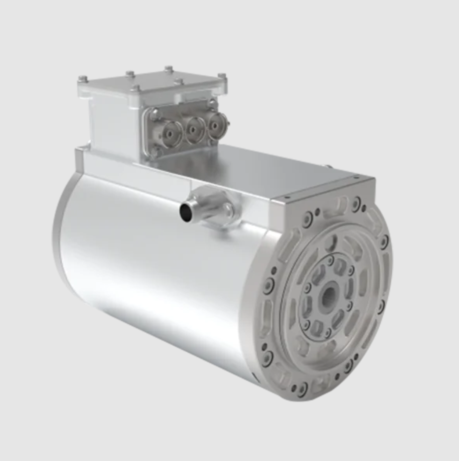
PMSM Electric Motor Fundamentals
The PMSM electric motor operates by synchronizing the rotor magnetic field with the rotating stator field. When three-phase alternating currents with a phase difference of 120 electrical degrees are supplied to the stator windings, a rotating magnetomotive force is produced. The rotor permanent magnets interact with this field, and electromagnetic torque is generated. Because the rotor has no excitation winding, the PMSM electric motor avoids rotor copper loss and can achieve very high efficiency. The synchronous speed is determined by the stator electrical frequency and the pole pair number:
$$
n_s = \frac{60 f_s}{p}
$$
where n_s is the synchronous speed in revolutions per minute, f_s is the stator frequency in hertz, and p is the number of pole pairs. The electrical angular speed and mechanical angular speed are related by:
$$
\omega_e = p \omega_m
$$
For the PMSM electric motor, the electromagnetic torque can be expressed in the d-q reference frame as:
$$
T_e = \frac{3}{2} p \left[ \psi_f i_q + (L_d – L_q) i_d i_q \right]
$$
In this equation, psi_f is the permanent magnet flux linkage, i_d and i_q are the d-axis and q-axis currents, and L_d and L_q are the d-axis and q-axis inductances. The first term is the permanent magnet torque, while the second term is the reluctance torque. For a surface-mounted PMSM electric motor, L_d is approximately equal to L_q, so the reluctance torque is small and the torque is almost proportional to i_q. For an interior-mounted PMSM electric motor, L_q is usually larger than L_d, so reluctance torque can be used to improve torque production and efficiency.
The steady-state voltage equations of the PMSM electric motor in the d-q frame are important for control design:
$$
v_d = R_s i_d – \omega_e L_q i_q
$$
$$
v_q = R_s i_q + \omega_e (L_d i_d + \psi_f)
$$
The dynamic voltage equations include the derivative terms:
$$
v_d = R_s i_d + L_d \frac{di_d}{dt} – \omega_e L_q i_q
$$
$$
v_q = R_s i_q + L_q \frac{di_q}{dt} + \omega_e (L_d i_d + \psi_f)
$$
These equations show that the d-axis and q-axis are coupled through the speed-dependent terms. For this reason, a PMSM electric motor controller must decouple the current loops or compensate for cross-coupling. Otherwise, the current response becomes sluggish, torque ripple increases, and high-speed operation becomes unstable.
The electromagnetic power and mechanical power relationship can be written as:
$$
P_{em} = T_e \omega_m
$$
Copper loss in the stator is approximated by:
$$
P_{cu} = \frac{3}{2} R_s (i_d^2 + i_q^2)
$$
Because copper loss is proportional to the square of current, the distribution of d-axis and q-axis current has a direct effect on efficiency. This is the main reason I consider maximum torque per ampere control so important for the PMSM electric motor in low-speed and high-torque conditions.
Comparison of PMSM Electric Motor Structures
| Feature | Surface-Mounted PMSM Electric Motor | Interior-Mounted PMSM Electric Motor |
|---|---|---|
| Rotor magnet position | Magnets mounted on rotor surface | Magnets embedded inside rotor core |
| Saliency | Low saliency, L_d approximately equal to L_q | High saliency, L_q usually greater than L_d |
| Reluctance torque | Small or negligible | Significant and usable |
| Mechanical strength | Lower, especially at high speed | Higher, suitable for high-speed operation |
| Field weakening capability | Limited | Better because d-axis current can weaken flux |
| Manufacturing cost | Generally lower | Higher due to magnet insertion and rotor complexity |
| Typical application | Low-speed and cost-sensitive PMSM electric motor drives | High-performance and wide-speed PMSM electric motor drives |
From my perspective, the interior-mounted PMSM electric motor is usually the stronger choice for traction because it can exploit reluctance torque, tolerate high-speed operation, and support field weakening. However, the surface-mounted PMSM electric motor remains attractive where smooth torque, simple control, and lower cost are more important than extreme speed range.
Performance Advantages of the PMSM Electric Motor
The PMSM electric motor offers several advantages over induction machines in electric vehicle traction. Because the rotor field is provided by permanent magnets, there is no rotor excitation current and no rotor copper loss. This improves efficiency, especially in part-load operation. The use of high-energy permanent magnets also enables high torque density and power density, which reduces machine volume and mass. With field-oriented control and field weakening, the PMSM electric motor can achieve a wide constant-power speed range. Its torque response is fast because the torque is primarily controlled by q-axis current. The thermal behavior is also favorable because rotor loss is low, although stator copper loss and inverter loss still require careful thermal management.
| Comparison Item | PMSM Electric Motor | Induction Motor |
|---|---|---|
| Rotor excitation | Permanent magnet | Induced rotor current |
| Rotor copper loss | Very low | Present |
| Efficiency at rated condition | High | Moderate to high |
| Power density | High | Moderate |
| Torque response | Fast | Relatively slower due to rotor flux dynamics |
| Field weakening | Possible but requires careful control | Natural through rotor slip |
| Control complexity | High | Moderate to high |
| Cost sensitivity | Affected by magnet price | Less affected by rare-earth materials |
For these reasons, I treat the PMSM electric motor as a primary candidate for high-performance electric vehicle traction. The main challenge is not the machine itself but the control strategy that must coordinate inverter voltage, current limits, speed, torque demand, and thermal constraints.
Drive System Architecture of the PMSM Electric Motor
A complete PMSM electric motor drive system includes the machine, power inverter, controller, sensors, cooling system, and communication interface. The machine contains the stator core, three-phase windings, rotor permanent magnets, shaft, bearings, and housing. The inverter converts direct current from the battery into three-phase alternating current using a three-phase full-bridge topology. The controller executes field-oriented control, space vector pulse width modulation, current limiting, field weakening, and fault protection. Sensors provide rotor position, phase current, direct-current bus voltage, and temperature information. The cooling system removes heat from the stator windings, stator core, rotor, and power modules.
| Subsystem | Core Function | Key Parameters I Consider |
|---|---|---|
| PMSM electric motor body | Electromechanical energy conversion | Rated power 50-200 kW, rated torque 150-500 N·m, pole pairs, flux linkage |
| Power inverter | DC to AC conversion and current regulation | Switching frequency 10-20 kHz, efficiency 98%-99%, SiC or IGBT devices |
| Controller | Control algorithm execution and signal processing | Main frequency above 300 MHz, response time below 1 ms |
| Position sensor | Rotor angle measurement for field orientation | Accuracy about ±0.1 electrical degrees |
| Current sensor | Phase current feedback | Measurement error below 1% |
| Temperature sensor | Thermal protection and derating | Winding, magnet, and power module temperature limits |
| Cooling system | Heat removal and continuous power capability | Coolant flow, thermal resistance, ambient conditions |
In my design philosophy, the PMSM electric motor and inverter must be treated as one integrated system. A control strategy that works on a test bench may fail in a vehicle if inverter voltage drop, cable inductance, sensor delay, and thermal derating are not included. The controller must therefore use accurate machine parameters and robust compensation.
Field-Oriented Control of the PMSM Electric Motor
Field-oriented control is the foundation of high-performance PMSM electric motor control. The main idea is to transform the three-phase stationary frame into a rotating d-q frame aligned with the rotor flux. In this frame, the d-axis current controls flux and the q-axis current controls torque. The Clarke transformation converts three-phase currents into two-phase stationary components:
$$
\begin{bmatrix}
i_\alpha \\
i_\beta
\end{bmatrix}
=
\frac{2}{3}
\begin{bmatrix}
1 & -\frac{1}{2} & -\frac{1}{2} \\
0 & \frac{\sqrt{3}}{2} & -\frac{\sqrt{3}}{2}
\end{bmatrix}
\begin{bmatrix}
i_a \\
i_b \\
i_c
\end{bmatrix}
$$
The Park transformation then rotates the stationary frame into the rotor synchronous frame:
$$
\begin{bmatrix}
i_d \\
i_q
\end{bmatrix}
=
\begin{bmatrix}
\cos\theta_e & \sin\theta_e \\
-\sin\theta_e & \cos\theta_e
\end{bmatrix}
\begin{bmatrix}
i_\alpha \\
i_\beta
\end{bmatrix}
$$
The inverse Park transformation is equally important because the controller must convert voltage commands back into the stationary frame:
$$
\begin{bmatrix}
v_\alpha \\
v_\beta
\end{bmatrix}
=
\begin{bmatrix}
\cos\theta_e & -\sin\theta_e \\
\sin\theta_e & \cos\theta_e
\end{bmatrix}
\begin{bmatrix}
v_d \\
v_q
\end{bmatrix}
$$
After inverse Clarke transformation, the voltage commands are used by space vector pulse width modulation to generate switching signals for the inverter. This structure allows the PMSM electric motor to behave like a separately excited direct-current machine, where torque and flux are controlled independently.
| Control Layer | Input | Output | Main Purpose |
|---|---|---|---|
| Speed loop | Speed reference and actual speed | q-axis current reference | Track vehicle speed or motor speed demand |
| d-axis current loop | d-axis current reference and feedback | d-axis voltage command | Control flux and field weakening |
| q-axis current loop | q-axis current reference and feedback | q-axis voltage command | Control torque production |
| Decoupling compensation | Speed, inductances, flux linkage | Feedforward voltage terms | Cancel cross-coupling between d and q axes |
| SVPWM | voltage commands in stationary frame | Inverter switching signals | Generate three-phase voltages |
The current loops are usually implemented with proportional-integral regulators. For the d-axis, I can write:
$$
v_d^* = K_{p,d}(i_d^* – i_d) + K_{i,d} \int (i_d^* – i_d) dt – \omega_e L_q i_q
$$
For the q-axis, the corresponding expression is:
$$
v_q^* = K_{p,q}(i_q^* – i_q) + K_{i,q} \int (i_q^* – i_q) dt + \omega_e (L_d i_d + \psi_f)
$$
The feedforward terms compensate for the coupling between the axes. Without them, a step change in q-axis current would disturb the d-axis current, and a change in d-axis current would disturb the q-axis current. The speed loop can be expressed as:
$$
i_q^* = K_{p,\omega}(\omega^* – \omega) + K_{i,\omega} \int (\omega^* – \omega) dt
$$
In my view, the speed loop should not be tuned too aggressively because the vehicle drivetrain includes backlash, tire slip, and a large equivalent inertia. A well-damped speed response is more important than an extremely fast response that causes torque oscillation. The PMSM electric motor can respond quickly, but the mechanical system and tire-road contact impose practical limits.
Maximum Torque Per Ampere Control Below Base Speed
Below base speed, the inverter voltage limit is not the dominant constraint. The main objective is to produce the required torque with the smallest possible current. This reduces copper loss and thermal stress. For the PMSM electric motor, this is called maximum torque per ampere control. The optimization problem can be stated as:
$$
\min I_s = \sqrt{i_d^2 + i_q^2}
$$
subject to the torque constraint:
$$
T_e = \frac{3}{2} p \left[ \psi_f i_q + (L_d – L_q) i_d i_q \right] = T^*
$$
Using a Lagrange multiplier, the stationary condition leads to the MTPA relationship. For an interior-mounted PMSM electric motor with L_q greater than L_d, the d-axis current reference can be expressed as:
$$
i_d^* = \frac{\psi_f – \sqrt{\psi_f^2 + 4(L_q – L_d)^2 i_q^2}}{2(L_q – L_d)}
$$
For a surface-mounted PMSM electric motor, where L_d is almost equal to L_q, the MTPA condition becomes:
$$
i_d^* = 0
$$
This means that for a surface-mounted PMSM electric motor, the best torque per ampere is obtained by using only q-axis current, provided that field weakening is not required. For an interior-mounted PMSM electric motor, a negative d-axis current is beneficial because it uses reluctance torque. The exact current distribution depends on the saliency ratio and the operating point.
| Operating Condition | Main Limit | Preferred Current Distribution | Control Objective |
|---|---|---|---|
| Low-speed launch | Current and thermal limits | MTPA, negative i_d for IPM | Maximum torque per ampere and smooth acceleration |
| Hill climbing | Continuous torque and temperature | MTPA with thermal derating | Reliable gradeability without overheating |
| Urban stop-and-go | Efficiency and response | MTPA with torque smoothing | Low energy consumption and low torque ripple |
| Base-speed transition | Voltage and current limits | MTPA to field weakening blend | Seamless mode transfer |
I have found that MTPA control gives the PMSM electric motor a strong advantage in low-speed drivability. During launch, the torque demand changes quickly, and the controller must avoid excessive current while still delivering enough torque to accelerate the vehicle. If the current distribution is poor, copper loss increases rapidly, the inverter heats up, and the available torque may be derated. MTPA reduces this risk by making better use of the magnetic and reluctance torque components.
Voltage and Current Limits Above Base Speed
Above base speed, the back electromotive force of the PMSM electric motor increases with speed. The inverter has a finite direct-current bus voltage, so the available alternating-current voltage is limited. The voltage limit can be approximated as:
$$
v_d^2 + v_q^2 \le V_{max}^2
$$
Neglecting stator resistance, the steady-state voltage constraint becomes:
$$
(L_d i_d + \psi_f)^2 + (L_q i_q)^2 \le \left( \frac{V_{max}}{\omega_e} \right)^2
$$
The current limit is given by:
$$
i_d^2 + i_q^2 \le I_{max}^2
$$
These two constraints define the feasible operating region. At low speed, the voltage limit is large, so the current limit dominates. At high speed, the voltage limit shrinks, and the PMSM electric motor must reduce flux to continue accelerating. This is achieved by applying negative d-axis current, which opposes the permanent magnet flux. The process is called field weakening or flux weakening.
Voltage Feedforward Field Weakening
Voltage feedforward field weakening predicts the voltage limit from speed and current references. When the controller detects that the required voltage is approaching the maximum inverter voltage, it adds a negative d-axis current component. A simple expression for the field-weakening d-axis current reference is:
$$
i_d^{fw} = -\frac{\psi_f}{L_d} + \frac{1}{L_d} \sqrt{ \left( \frac{V_{max}}{\omega_e} \right)^2 – (L_q i_q)^2 }
$$
This equation shows that as speed increases, the allowable voltage term V_max/omega_e decreases. To keep the square root real, i_q may also need to be reduced. The controller therefore coordinates the d-axis and q-axis references. A feedforward correction can be written as:
$$
i_d^* = i_d^{MTPA} + i_d^{fw}
$$
In practice, the field-weakening term must be limited to avoid excessive current and demagnetization risk. I also include a voltage margin because the inverter has dead time, device voltage drop, and modulation limits. The margin prevents the controller from operating exactly at the voltage boundary, where small disturbances can cause loss of current control.
| Field-Weakening Method | Main Principle | Strength | Risk I Must Manage |
|---|---|---|---|
| Voltage feedforward field weakening | Predict voltage limit and add negative i_d | Fast response and smooth transition | Parameter sensitivity and voltage margin |
| Current limiting field weakening | Respect maximum current while weakening flux | Protects inverter and motor windings | Torque reduction at very high speed |
| Lookup-table field weakening | Use calibrated maps for i_d and i_q | Simple real-time implementation | Requires extensive calibration |
| Model-based field weakening | Solve voltage and current constraints online | Adapts to operating conditions | Higher computational load |
Current Limiting Field Weakening
Current limiting field weakening protects the inverter and the PMSM electric motor when the current magnitude approaches the maximum limit. If the current vector exceeds the limit, the controller must reduce the q-axis current or adjust the d-axis current. The current limit circle is:
$$
i_d^2 + i_q^2 = I_{max}^2
$$
For a given q-axis current, the maximum negative d-axis current allowed by the current limit is:
$$
i_d^{max} = -\sqrt{I_{max}^2 – i_q^2}
$$
When the voltage limit and current limit intersect, the PMSM electric motor operates at the corner of the feasible region. In this region, the controller cannot increase torque without exceeding either voltage or current. The control strategy must then prioritize safety and stability. I usually set the current limit slightly below the hardware limit and use a thermal model to reduce it further when temperatures rise.
The combined voltage and current limit problem can be expressed as:
$$
\max T_e
$$
subject to:
$$
i_d^2 + i_q^2 \le I_{max}^2
$$
$$
(L_d i_d + \psi_f)^2 + (L_q i_q)^2 \le \left( \frac{V_{max}}{\omega_e} \right)^2
$$
This is a constrained optimization problem. In real-time control, I solve it approximately using feedforward terms, lookup tables, and feedback correction. The goal is not to find a perfect mathematical solution every switching period, but to maintain stable torque, current, and voltage behavior across the entire speed range.
| Speed Region | Dominant Constraint | Current Strategy | Expected Behavior |
|---|---|---|---|
| Low speed | Current and thermal limits | MTPA | High torque per ampere, strong launch |
| Medium speed | Voltage limit begins to appear | MTPA with mild field weakening | Smooth transition to constant power |
| Base speed | Voltage and current limits intersect | Field weakening enters actively | Maximum power at rated voltage |
| High speed | Voltage limit dominates | Negative i_d and reduced i_q | Wide speed range with reduced torque |
| Very high speed | Voltage limit and thermal derating | Current-limited field weakening | Safe operation with limited torque |
Integrated Control Architecture for the PMSM Electric Motor
In my view, a practical PMSM electric motor controller should combine several layers. The highest layer interprets the driver torque demand, vehicle speed, battery state, and thermal state. The middle layer selects the operating mode, such as MTPA, field weakening, derating, or fault mode. The lowest layer executes current control and pulse width modulation. This hierarchy allows the controller to protect the hardware while still delivering the requested torque whenever possible.
| Layer | Function | Typical Time Scale |
|---|---|---|
| Vehicle supervisory control | Torque demand interpretation and energy management | 10-100 ms |
| Mode selection | MTPA, field weakening, derating, fault response | 1-10 ms |
| Speed and torque control | Generate current references | 0.1-1 ms |
| Current control | Regulate i_d and i_q | 50-200 microseconds |
| PWM and gate drive | Generate switching signals | Switching period |
I also include a parameter adaptation block. The PMSM electric motor parameters, especially stator resistance and permanent magnet flux linkage, change with temperature. If the controller uses fixed parameters, the decoupling terms and field-weakening references become inaccurate. Temperature compensation improves torque accuracy and prevents unexpected current errors at high temperature.
Case Study: Integrated Electric Drive with a PMSM Electric Motor
I now consider a highly integrated multi-in-one electric drive system that uses a PMSM electric motor. The system combines the motor, inverter, controller, and some vehicle control functions. The power module uses advanced interconnection and thermal design to improve heat dissipation. The control strategy uses a speed-current dual-loop structure with field-oriented control. The outer loop generates the speed or torque command, and the inner loop regulates d-axis and q-axis current. The rotor position is used for field orientation, and space vector pulse width modulation generates the inverter switching signals.
The test configuration I use for analysis is summarized below. The values are representative of a traction PMSM electric motor in a light commercial vehicle or premium passenger car.
| Parameter | Value | Unit |
|---|---|---|
| Rated power | 120 | kW |
| Peak power | 180 | kW |
| Rated torque | 300 | N·m |
| Peak torque | 450 | N·m |
| DC bus voltage | 400 | V |
| Switching frequency | 12 | kHz |
| Pole pairs | 4 | – |
| Permanent magnet flux linkage | 0.12 | Wb |
| d-axis inductance | 0.00025 | H |
| q-axis inductance | 0.00050 | H |
| Maximum current | 400 | A |
I evaluate five operating scenarios: launch, hill climb, urban driving, highway cruising, and regenerative braking. In each scenario, the PMSM electric motor control strategy must balance torque, efficiency, voltage, current, and temperature. The following table summarizes the expected control focus and performance outcome.
| Scenario | Control Focus | PMSM Electric Motor Behavior | Performance Outcome |
|---|---|---|---|
| Launch | MTPA and current limiting | High q-axis current, negative d-axis current for IPM | Fast acceleration with controlled copper loss |
| Hill climb | Continuous torque and thermal derating | MTPA with temperature-based current reduction | Stable gradeability without overheating |
| Urban driving | Efficiency and torque smoothness | Frequent torque reversal, low ripple | Low energy consumption and comfortable drivability |
| Highway cruising | Field weakening and voltage margin | Negative d-axis current, reduced q-axis current | Wide speed range and stable power delivery |
| Regenerative braking | Torque reversal and current limit | Negative q-axis current, voltage control | Energy recovery with safe bus voltage |
From my analysis, the integrated drive shows clear improvements when MTPA and field weakening are coordinated. At low speed, the PMSM electric motor produces high torque per ampere, so the inverter current is lower for the same torque. At high speed, voltage feedforward field weakening prevents voltage saturation, and current limiting field weakening protects the power devices. The transition between these modes is critical. If the transition is too abrupt, torque ripple and current spikes appear. If it is too slow, the vehicle may lose acceleration or the inverter may enter voltage saturation.
Performance Comparison of Control Strategies
To compare control strategies, I use several metrics: torque response time, torque ripple, efficiency at low speed, efficiency at high speed, maximum speed capability, and thermal stress. The table below presents a qualitative and semi-quantitative comparison based on my evaluation.
| Control Strategy | Torque Response | Torque Ripple | Low-Speed Efficiency | High-Speed Efficiency | Speed Range | Thermal Stress |
|---|---|---|---|---|---|---|
| Simple i_d = 0 control | Good | Moderate | Moderate for IPM | Poor without field weakening | Limited | High at high torque |
| MTPA control | Excellent | Low | Excellent | Not sufficient alone | Base speed only | Reduced at low speed |
| Voltage feedforward field weakening | Very good | Low to moderate | Good | Very good | Wide | Moderate |
| Current limiting field weakening | Good | Low | Good | Good | Wide and protected | Low due to current protection |
| Combined MTPA and field weakening | Excellent | Low | Excellent | Very good | Very wide | Well managed |
I find that the combined strategy is the most suitable for the PMSM electric motor in electric vehicles. MTPA ensures high torque per ampere below base speed, while field weakening extends the speed range above base speed. The controller must blend the two strategies according to the voltage and current limits. A smooth blending function can be written as:
$$
\alpha = \frac{1}{1 + e^{-k(\omega_e – \omega_{b})}}
$$
where alpha is the blending factor and omega_b is the base speed. The d-axis current reference can then be expressed as:
$$
i_d^* = (1 – \alpha) i_d^{MTPA} + \alpha i_d^{FW}
$$
This logistic blending avoids sudden mode changes. I prefer this approach because it reduces torque ripple during the transition from constant-torque to constant-power operation.
Efficiency and Loss Analysis
The efficiency of the PMSM electric motor depends on copper loss, iron loss, mechanical loss, stray loss, and inverter loss. In my analysis, copper loss is the most sensitive to current distribution, so MTPA is effective at low speed. Iron loss increases with electrical frequency, so high-speed operation requires field weakening and sometimes active derating. Inverter loss includes conduction loss and switching loss. Increasing switching frequency reduces current ripple but increases switching loss. Therefore, the controller should use the lowest switching frequency that satisfies torque ripple and acoustic requirements.
| Loss Component | Main Dependence | Control Lever |
|---|---|---|
| Stator copper loss | Current squared | MTPA, current limiting, thermal derating |
| Stator iron loss | Electrical frequency and flux | Field weakening, flux reference shaping |
| Rotor loss | Harmonics and eddy currents | Current harmonic reduction, PWM optimization |
| Inverter conduction loss | Current magnitude | MTPA, reduced current for same torque |
| Inverter switching loss | Switching frequency and DC voltage | Modulation strategy and switching frequency selection |
| Mechanical loss | Speed and bearing friction | Speed planning and regenerative control |
I also note that the PMSM electric motor can suffer from additional losses if the current contains harmonics. Field-oriented control with space vector pulse width modulation reduces low-order harmonics, but dead time, sensor offset, and inverter nonlinearity can still cause torque ripple. Compensation algorithms for dead time and voltage drop improve current waveform quality and reduce loss.
Thermal Management and Derating
Thermal management is a key part of PMSM electric motor control. The stator winding temperature, permanent magnet temperature, and power module temperature must be monitored. If any temperature exceeds a threshold, the controller should reduce current or torque. A simple derating function can be written as:
$$
k_T =
\begin{cases}
1, & T \le T_{low} \\
\frac{T_{high} – T}{T_{high} – T_{low}}, & T_{low} < T < T_{high} \\
0, & T \ge T_{high}
\end{cases}
$$
The torque limit is then:
$$
T_{max}^{derated} = k_T T_{max}
$$
I use this kind of derating in my control architecture because it protects the PMSM electric motor and inverter during prolonged hill climbing or high-speed driving. The derating should be gradual, not abrupt, to avoid an uncomfortable torque drop. A thermal observer can estimate temperatures that are not directly measured, such as magnet temperature, and improve protection.
| Thermal Condition | Control Response | Effect on PMSM Electric Motor |
|---|---|---|
| Normal temperature | Full torque and MTPA | High performance and efficiency |
| Winding temperature rising | Reduce continuous current limit | Lower copper loss and slower heating |
| Power module temperature rising | Reduce switching frequency or current | Lower inverter loss and safer operation |
| Magnet temperature high | Limit negative d-axis current | Reduce demagnetization risk |
| Severe over-temperature | Torque derating or shutdown | Protect hardware and ensure safety |
Sensor and Observer Considerations
Field-oriented control requires rotor position. A position sensor provides accurate angle information, but it adds cost and wiring. Sensorless control can estimate rotor position from voltage and current, but at low speed the back electromotive force is small, so estimation becomes difficult. In my opinion, a practical PMSM electric motor drive can use a hybrid approach: sensored control at low speed and sensorless control at high speed. This reduces cost while maintaining performance.
| Method | Low-Speed Performance | High-Speed Performance | Cost and Complexity |
|---|---|---|---|
| Resolver or encoder | Excellent | Excellent | Higher cost and wiring |
| Hall sensors | Moderate | Good with interpolation | Moderate cost |
| High-frequency injection sensorless | Good for salient PMSM electric motor | Less suitable | High computational load |
| Back-EMF observer sensorless | Poor at very low speed | Excellent | Moderate complexity |
| Hybrid sensored and sensorless | Good | Excellent | Balanced cost and performance |
Fault Tolerance and Reliability
Reliability is essential for the PMSM electric motor in vehicle traction. Faults can include current sensor failure, position sensor failure, inverter switch failure, overvoltage, overcurrent, and overheating. The controller should detect faults quickly and transition to a safe state. For example, if one phase current sensor fails, the controller can estimate current from the other phases if the neutral point is isolated. If the position sensor fails, the controller can switch to sensorless estimation or a limp-home mode. If a power switch fails, the inverter can enter a controlled shutdown or use redundant phases if the topology allows.
| Fault | Detection Method | Safe Response |
|---|---|---|
| Overcurrent | Current sensor and comparator | Pulse width modulation shutdown, current limit |
| Overvoltage | DC bus voltage measurement | Regenerative torque reduction, brake chopper if available |
| Position sensor fault | Signal plausibility and observer residual | Sensorless fallback or limp-home mode |
| Power switch fault | Desaturation detection and phase current analysis | Controlled shutdown or fault-tolerant operation |
| Over-temperature | Temperature sensors and thermal model | Derating and cooling request |
In my design reviews, I emphasize that the PMSM electric motor control strategy must be robust to parameter variation. Stator resistance changes with temperature, permanent magnet flux linkage decreases with temperature, and inductance varies with current due to magnetic saturation. If the controller ignores these effects, the MTPA trajectory and field-weakening boundary become inaccurate. Online parameter estimation or lookup-table compensation can reduce this error.
Practical Tuning Procedure I Use
When I tune a PMSM electric motor control system, I follow a step-by-step procedure. First, I verify the rotor position offset and phase sequence. Second, I measure stator resistance and inductance at several current levels. Third, I tune the d-axis and q-axis current loops with the motor locked or at low speed. Fourth, I tune the speed loop with a representative load inertia. Fifth, I calibrate the MTPA table or equation. Sixth, I calibrate the field-weakening table and voltage margin. Seventh, I test transitions between MTPA and field weakening. Finally, I validate thermal derating and fault responses.
| Tuning Step | Purpose | Key Check |
|---|---|---|
| Position offset calibration | Align d-q frame with rotor flux | Zero torque at i_d current and zero i_q |
| Current loop tuning | Achieve fast and stable current response | No overshoot and no cross-coupling |
| Speed loop tuning | Match vehicle inertia and drivability | Well-damped response to torque step |
| MTPA calibration | Minimize current for given torque | Low copper loss and correct torque |
| Field-weakening calibration | Extend speed range safely | Voltage margin and no current overshoot |
| Thermal validation | Confirm derating behavior | Stable temperature under load cycles |
Comparative Dynamic Response
I summarize the dynamic response of the PMSM electric motor under different control modes in the next table. The values are normalized for comparison. A value of 1.0 means the best performance among the compared modes.
| Metric | i_d = 0 | MTPA | Field Weakening | Combined MTPA and Field Weakening |
|---|---|---|---|---|
| Torque response speed | 0.85 | 0.95 | 0.80 | 0.95 |
| Torque ripple quality | 0.75 | 0.90 | 0.80 | 0.92 |
| Low-speed efficiency | 0.70 | 0.98 | 0.65 | 0.96 |
| High-speed efficiency | 0.55 | 0.60 | 0.90 | 0.93 |
| Maximum speed capability | 0.50 | 0.55 | 0.95 | 0.98 |
| Thermal robustness | 0.70 | 0.88 | 0.85 | 0.94 |
These normalized results support my conclusion that no single control mode is sufficient. The PMSM electric motor must switch or blend control modes based on speed, voltage, current, and temperature. The combined strategy gives the best overall balance.
Modeling and Simulation Approach
For simulation, I use a d-q model of the PMSM electric motor with parameter tables for inductance and flux linkage. The inverter is modeled with switching behavior or an average model depending on the study. The vehicle model includes mass, drag, rolling resistance, and gear ratio. The control model includes field-oriented control, MTPA, field weakening, current limiting, and thermal derating. I run test cycles such as low-speed launch, grade climbing, urban stop-and-go, and highway cruising. I then compare current magnitude, torque, speed, voltage, and efficiency.
| Model Block | Key Variables | Purpose |
|---|---|---|
| PMSM electric motor d-q model | i_d, i_q, v_d, v_q, omega_e | Electromagnetic torque and current dynamics |
| Inverter model | DC bus voltage, switching signals | Voltage and current limit representation |
| Control model | Speed reference, current reference | FOC, MTPA, field weakening |
| Vehicle model | Mass, speed, grade, drag | Load torque calculation |
| Thermal model | Winding and magnet temperature | Derating and protection |
Key Observations from My Analysis
First, the PMSM electric motor requires accurate rotor position for field orientation. Any angle error reduces torque per ampere and can cause instability. Second, MTPA is essential below base speed because it reduces current and copper loss for a given torque. Third, field weakening is essential above base speed because it prevents voltage saturation. Fourth, current limiting field weakening is necessary to protect the inverter and windings. Fifth, thermal derating must be integrated with torque control to avoid overheating. Sixth, smooth mode transitions are critical for drivability and torque quality.
I also observe that the PMSM electric motor performs best when the control strategy is matched to the rotor topology. For a surface-mounted PMSM electric motor, the controller can use i_d equal to zero below base speed and rely on field weakening at high speed. For an interior-mounted PMSM electric motor, the controller should use reluctance torque through negative i_d and optimize the current trajectory. This distinction is often overlooked in simple controllers, but it has a major effect on efficiency and torque capability.
| Observation | Implication for PMSM Electric Motor Control |
|---|---|
| Parameter variation with temperature | Use compensation for resistance and flux linkage |
| Magnetic saturation | Use current-dependent inductance tables |
| Inverter nonlinearity | Compensate dead time and voltage drop |
| Field-weakening voltage margin | Prevent voltage saturation and current loss |
| Thermal derating | Protect magnets and windings during high load |
| Mode transition | Blend MTPA and field weakening smoothly |
Conclusion
In my final assessment, the PMSM electric motor is a strong foundation for electric vehicle traction because it offers high efficiency, high power density, fast torque response, and a wide speed range when controlled properly. Field-oriented control provides the basic decoupled control structure. Maximum torque per ampere control improves low-speed and high-torque operation by minimizing current and copper loss. Voltage feedforward field weakening and current limiting field weakening extend the high-speed range while protecting the inverter and the machine. An integrated control architecture that blends these strategies, compensates for parameter variation, and respects thermal limits can significantly improve the dynamic response and energy efficiency of the PMSM electric motor.
I therefore recommend a combined control approach: use MTPA below base speed, use voltage and current constrained field weakening above base speed, use smooth blending between modes, and use thermal derating as a supervisory constraint. With this approach, the PMSM electric motor can deliver strong launch performance, stable hill climbing, low urban energy consumption, reliable highway cruising, and safe regenerative braking. The result is a traction system that is not only powerful but also efficient, durable, and suitable for the demanding operating conditions of modern electric vehicles.