
As an engineer and researcher deeply involved in vehicle engineering, I have dedicated significant effort to understanding and improving the remaining range prediction systems in battery electric vehicles. The accuracy of remaining range prediction is not merely a technical metric; it is intrinsically tied to user confidence and overall driving experience. Early battery electric vehicles often relied on single-algorithm approaches, which frequently led to inaccurate predictions, exacerbating what is commonly known as “range anxiety.” This article, written from my first-person perspective, explores the transformative potential of multi-algorithm fusion. I will comprehensively analyze the core factors influencing prediction accuracy, critically examine the limitations of existing single algorithms, and detail practical application paths for multi-algorithm fusion. My goal is to provide a roadmap for significantly enhancing the precision of remaining range predictions in battery electric vehicles, thereby fostering greater user trust and adoption.
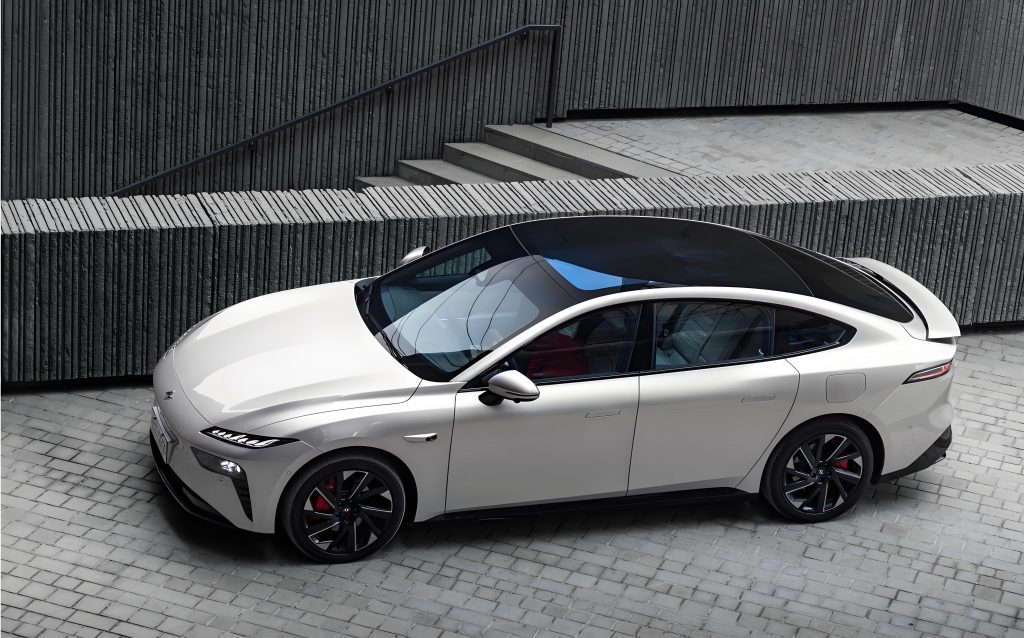
Core Factors Influencing Remaining Range in Battery Electric Vehicles
The prediction of remaining range in a battery electric vehicle is a complex estimation problem influenced by a dynamic interplay of multiple factors. From my analysis, these factors can be systematically categorized into four primary domains: battery state, vehicle state, driving behavior, and the surrounding environment. Each domain encompasses specific variables that directly affect energy consumption rates and, consequently, the distance a battery electric vehicle can travel on its remaining charge. Understanding these factors is the foundational step toward developing robust prediction models.
The battery, being the sole energy source for a battery electric vehicle, is the most critical component. Its state is characterized by several key indicators. The State of Charge (SOC) represents the instantaneous available energy and serves as the primary input for range calculation. However, SOC estimation is prone to errors, especially under low-temperature conditions where measured values can deviate from actual capacity. The State of Health (SOH) reflects the battery’s aging and capacity fade over time, a crucial factor for long-term range accuracy. Battery temperature drastically influences electrochemical activity; low temperatures reduce available capacity, while high temperatures increase auxiliary cooling load and accelerate degradation. Finally, battery consistency—the performance variation among individual cells—determines the pack’s effective usable capacity. These relationships can be summarized mathematically. For instance, the effective battery capacity $C_{eff}$ considering SOH and temperature factor $f(T)$ can be expressed as:
$$C_{eff} = C_{rated} \times SOH \times f(T)$$
where $C_{rated}$ is the nominal capacity. The function $f(T)$ is typically less than 1 at temperature extremes. A comprehensive summary of battery state factors is provided below.
| Factor | Symbol | Description | Mathematical Relation & Impact |
|---|---|---|---|
| State of Charge | SOC | Instantaneous remaining capacity as a percentage of total capacity. | $$SOC(t) = \frac{Q_{remain}(t)}{C_{eff}}$$ Base for range calculation; estimation error directly propagates to range error. |
| State of Health | SOH | Ratio of current maximum capacity to initial rated capacity. | $$SOH = \frac{C_{current\_max}}{C_{rated}}$$ Long-term capacity fade reduces total energy available, causing range shrinkage over vehicle life. |
| Battery Temperature | T_batt | Operating temperature of the battery pack. | Affects internal resistance $R_{int}(T)$ and open-circuit voltage $V_{oc}(T)$. Low $T_batt$ increases $R_{int}$, reducing usable capacity and power. |
| Battery Consistency | σ | Standard deviation of capacity or impedance across cells. | High σ reduces total usable capacity to that of the weakest cell: $C_{usable} = min(C_{cell\_1}, C_{cell\_2}, …)$. Increases risk of premature shutdown. |
The vehicle’s operational state is another major determinant of energy efficiency for any battery electric vehicle. This includes both the physical condition of hardware and the usage of auxiliary systems. For example, under-inflated tires increase rolling resistance, a misaligned chassis induces drag, and a dragging brake system wastes energy. The vehicle load, including passengers and cargo, directly increases the mass, which elevates the energy required for acceleration and hill climbing. Furthermore, comfort features like air conditioning, heating, and infotainment systems draw significant power from the high-voltage battery. The instantaneous auxiliary power demand $P_{aux}(t)$ can be a substantial fraction of the total load. The total instantaneous power consumption $P_{total}(t)$ of a battery electric vehicle can be modeled as:
$$P_{total}(t) = P_{prop}(t) + P_{aux}(t)$$
where $P_{prop}(t)$ is the propulsion power related to driving dynamics.
| Category | Examples | Impact on Energy Consumption |
|---|---|---|
| Hardware State | Tire pressure, wheel alignment, brake drag, vehicle mass (load). | Increases rolling resistance ($F_{roll}$) and inertial mass ($m$), directly raising energy per distance: $$E_{mile} \propto (F_{roll} + ma + mg\sin\theta) \cdot d$$ |
| Auxiliary System Usage | Climate control, seat heating, headlights, multimedia. | Adds constant or variable power load $P_{aux}$. Range reduction ΔR ≈ $P_{aux} \cdot t_{drive} / (Efficiency \cdot Avg\_Consumption)$. |
Driver behavior introduces high variability into the energy consumption profile of a battery electric vehicle. Aggressive driving with frequent hard acceleration and braking is particularly inefficient. Hard acceleration demands high current from the battery, often operating it in less efficient regions, while hard braking may not allow for optimal regenerative energy recovery. In contrast, smooth, anticipatory driving maximizes efficiency. The impact can be quantified by comparing average energy consumption rates. Studies, including my own observations, indicate that aggressive driving can increase energy consumption by 20% to 35% compared to an eco-driving style. The kinetic energy lost during non-regenerative braking is $E_{loss} = \frac{1}{2} m v^2 \cdot (1-\eta_{regen})$, where $\eta_{regen}$ is the regenerative braking efficiency.
Finally, the surrounding environment poses external forces that a battery electric vehicle must overcome. Road grade is a dominant factor; climbing a hill requires work against gravity ($m g h$). Traffic congestion leads to frequent stop-and-go cycles, which are inherently inefficient. Road surface roughness increases rolling resistance. Environmental conditions like air density (affected by temperature and altitude) influence aerodynamic drag force, given by $F_{drag} = \frac{1}{2} \rho C_d A v^2$. Strong headwinds effectively increase $v$ in this equation. Adverse weather such as rain or snow not only increases rolling resistance but also forces the use of energy-intensive systems like wipers, defrosters, and headlights. The combined effect of these environmental factors can be modeled as an additional resistive force $F_{env}$.
Inherent Limitations of Single-Algorithm Prediction Methods
Historically, battery electric vehicles have employed various single-algorithm strategies for range prediction. While these methods laid the groundwork, my experience and research have consistently highlighted their fundamental limitations, which become pronounced in real-world, dynamic driving conditions.
Battery Model-Based Approaches
These methods rely on a mathematical representation of the battery to estimate SOC, which is then combined with an average or instantaneous energy consumption value to predict range. The two most common types are the Equivalent Circuit Model (ECM) and the Ampere-Hour (Ah) Integral method.
The Equivalent Circuit Model uses electrical components like resistors and capacitors to simulate battery dynamics. A first-order RC model, for instance, includes an open-circuit voltage source $V_{OC}(SOC)$, an internal resistance $R_0$, and an RC parallel network ($R_1, C_1$) to model polarization effects. The terminal voltage $V_t$ is given by:
$$V_t = V_{OC}(SOC) – I R_0 – V_1$$
where $\frac{dV_1}{dt} = \frac{I}{C_1} – \frac{V_1}{R_1 C_1}$. While theoretically sound, the ECM’s accuracy depends on precise, frequently updated parameters. The table below outlines its key limitations.
| Limitation | Technical Explanation | Consequence for Battery Electric Vehicle Prediction |
|---|---|---|
| Parameter Sensitivity & Calibration Burden | Model parameters ($R_0, R_1, C_1, V_{OC}(SOC)$) vary with SOC, temperature, aging, and load history. They require extensive lab characterization and online identification algorithms (e.g., Kalman Filters). | Incorrect or outdated parameters lead to SOC estimation drift, causing range prediction errors. The computational cost of online parameter identification strains vehicle ECUs. |
| Computational Complexity | Solving differential equations for SOC estimation and predicting future states under variable load is computationally intensive. | Leads to slower update rates or simplified models that sacrifice accuracy. Real-time prediction on resource-constrained hardware becomes challenging. |
The Ampere-Hour Integral method is simpler, calculating SOC by integrating the battery current $I(t)$:
$$SOC(t) = SOC(t_0) – \frac{1}{C_{nominal}} \int_{t_0}^{t} \eta(I) I(\tau) d\tau$$
where $\eta(I)$ is the coulombic efficiency. Its primary flaw is that it is an open-loop integrator. Any error in the initial SOC($t_0$), current sensor bias, or uncertainty in efficiency $\eta$ accumulates without bound over time. It also ignores the voltage-sag effect under load, which impacts available energy.
Driving Cycle and Machine Learning Approaches
These data-driven methods learn the relationship between driving patterns, context, and energy consumption from historical data. They can be very adaptive but come with their own set of challenges for deployment in battery electric vehicles.
| Algorithm Type | Basic Principle | Key Limitations |
|---|---|---|
| Driving Cycle Matching | Matches current driving (speed, acceleration) to pre-defined cycles with known energy consumption. | Fails in unseen or mixed driving conditions. Lacks generalizability. Requires a large, representative library of cycles. |
| Machine Learning (e.g., Neural Networks, Random Forest) | Maps features (speed, acceleration, temperature, auxiliary load) directly to energy consumption or range via trained models. | Data Hungry: Requires massive, high-quality, labeled datasets covering all possible scenarios. Black Box Nature: Poor interpretability makes validation and debugging difficult for safety-critical applications. Computational Demand: Training is offline, but inference may still be heavy for complex models on vehicle hardware. Overfitting Risk: Models may perform poorly on data from different geographic regions or driver populations. |
Empirical Formula Methods
These are simple, rule-based methods often derived from laboratory test data. A common form is:
$$R_{remaining} = \frac{SOC \times C_{nominal} \times V_{nominal}}{E_{avg}}$$
where $E_{avg}$ is a fixed average energy consumption per kilometer. The limitation is stark: $E_{avg}$ is not constant. It changes instantly with driver behavior, climate control use, and road grade. Therefore, such methods are only accurate under conditions identical to the test cycle, rendering them unreliable for real-world use in a battery electric vehicle.
In summary, while each single algorithm has merits, none possesses the robustness, accuracy, and adaptability required for reliable remaining range prediction across the diverse operating conditions of a modern battery electric vehicle. This realization has driven the shift towards multi-algorithm fusion.
Advanced Application Paths: Multi-Algorithm Fusion Architectures
To overcome the deficiencies of monolithic approaches, I advocate for and have researched multi-algorithm fusion frameworks. These architectures synergistically combine the strengths of different algorithms while mitigating their individual weaknesses. I will detail three primary fusion paths: weighted fusion, feature fusion, and stage fusion, each suited to different priorities and vehicle segments within the battery electric vehicle market.
1. Weighted Fusion Architecture
This is a relatively straightforward yet effective fusion strategy. Multiple prediction algorithms run in parallel, and their outputs are combined using a weighted sum. The core idea is to assign higher weights to algorithms that are more reliable under the current driving context. This method is particularly attractive for mass-market battery electric vehicles due to its implementational simplicity and moderate computational overhead.
The mathematical formulation is:
$$R_{final}(t) = \sum_{i=1}^{N} w_i(t) \cdot R_i(t)$$
subject to $\sum_{i=1}^{N} w_i(t) = 1$. Here, $R_i(t)$ is the remaining range predicted by the $i$-th algorithm, and $w_i(t)$ is its dynamically assigned weight at time $t$.
The critical intelligence lies in the dynamic weight allocation mechanism. Weights can be determined based on real-time confidence scores for each algorithm. Confidence can be estimated from factors such as:
– **Algorithm-Specific Error Metrics:** Short-term historical accuracy (e.g., comparing recent predictions with actual energy use).
– **Contextual Relevance:** How well the algorithm’s underlying model matches the current context (e.g., an ECM’s weight might be reduced if battery temperature is changing rapidly, exceeding its calibrated range).
– **Sensor Data Quality:** The reliability of the primary sensors feeding the algorithm (e.g., current sensor noise).
A rule-based or a simple machine learning model (e.g., a shallow neural network) can be used for this dynamic weighting. For instance, consider a system fusing an Equivalent Circuit Model (ECM), a driving pattern recognizer (DPR), and a simplified empirical model (EMP). The weight allocation might follow the logic summarized below:
| Driving Context | ECM Weight ($w_1$) | DPR Weight ($w_2$) | EMP Weight ($w_3$) | Rationale |
|---|---|---|---|---|
| Highway, Steady Speed | 0.2 | 0.7 | 0.1 | DPR excels in stable, predictable conditions. ECM is less critical. |
| Urban, Stop-and-Go | 0.6 | 0.3 | 0.1 | ECM better handles variable loads and regenerative braking. DPR struggles with unpredictability. |
| Extreme Cold (< 0°C) | 0.8 | 0.1 | 0.1 | ECM, if properly temperature-compensated, is most reliable. Other models lack detailed battery state knowledge. |
| Auxiliary Loads Very High | 0.4 | 0.5 | 0.1 | DPR trained on data with high auxiliary use may capture this well. ECM may not fully account for it. |
2. Feature Fusion Architecture
Feature fusion represents a deeper level of integration. Instead of combining final predictions, it combines the raw or processed input features from multiple sources or models at an early stage, feeding them into a single, powerful meta-model. This approach allows the model to discover complex, non-linear interactions between features that individual algorithms might miss. It is well-suited for premium or next-generation battery electric vehicles with more advanced sensor suites and computing platforms.
The process involves several key steps, which I have implemented in research prototypes:
Step 1: Multi-Modal Data Acquisition. A comprehensive sensor network collects data:
– **Battery Domain:** Cell voltages, pack current, module temperatures.
– **Vehicle Dynamics Domain:** Wheel speed, accelerator/brake pedal position, longitudinal/lateral acceleration.
– **Chassis Domain:** Wheel force sensors (if available), tire pressure monitoring system (TPMS) data.
– **Auxiliary System Domain:** Climate control compressor power, heater power, multimedia system status.
– **Environmental Domain:** Ambient temperature, barometric pressure, GPS data (for elevation and map matching), camera/radar data for traffic density estimation.
Step 2: Feature Engineering and Fusion. Raw signals are processed into meaningful features. For example, from velocity, we derive average speed, positive acceleration kinetic energy, and stop duration. Features from different domains are then concatenated into a unified feature vector $\mathbf{F}(t)$:
$$\mathbf{F}(t) = [\mathbf{F}_{batt}(t), \mathbf{F}_{drv}(t), \mathbf{F}_{aux}(t), \mathbf{F}_{env}(t)]^T$$
Dimensionality reduction techniques like Principal Component Analysis (PCA) or feature selection algorithms can be applied to manage complexity and reduce noise.
Step 3: Meta-Model Training and Prediction. The fused feature vector $\mathbf{F}(t)$ is fed into a sophisticated machine learning model, such as a Gradient Boosting Regressor (e.g., XGBoost) or a Recurrent Neural Network (RNN). This model is trained end-to-end to predict either instantaneous energy consumption or directly the remaining range. The training objective is typically to minimize the Mean Absolute Percentage Error (MAPE) on the range. The model can be represented as:
$$R_{remaining}(t) = M_{\theta}(\mathbf{F}(t), SOC(t))$$
where $M_{\theta}$ is the meta-model with parameters $\theta$. This architecture’s strength is its ability to learn directly from correlated multi-domain data, leading to high accuracy but at the cost of requiring significant offline training and online computational resources.
3. Stage Fusion Architecture
This architecture adopts a temporal, hierarchical perspective. It recognizes that the prediction horizon significantly influences the choice of the best algorithm. A battery electric vehicle driver needs instant feedback (short-term), a reliable estimate for the next hour of driving (medium-term), and a planning estimate for a full trip (long-term). Stage fusion assigns different algorithms to these different horizons.
Short-Term Prediction (Seconds to Minutes): Focus: **Timeliness and Reactivity.** The primary goal is to react instantly to driver inputs. This layer often uses a physics-based instantaneous model or a filtered version of the Ah integral. A simple but effective short-term model calculates range from current power draw:
$$R_{short}(t) = \frac{SOC(t) \times C_{eff} \times V_{nominal}}{P_{total}(t) / v(t)}$$
where $P_{total}(t)/v(t)$ is the instantaneous energy consumption per km. This is updated several times per second.
Medium-Term Prediction (Minutes to ~1 Hour): Focus: **Reliability and Trend Awareness.** This layer integrates information over a recent time window to smooth out noise and account for trends. A Kalman Filter combining an ECM for SOC estimation with a driving pattern-based energy consumption predictor works well here. It provides a stable and more accurate estimate than the short-term layer.
Long-Term Prediction (1 Hour to End of Trip): Focus: **Anticipatory Planning and Environmental Adaptation.** This layer incorporates route information (from navigation), elevation profile, forecast weather, and typical traffic patterns for the planned route. It employs machine learning or advanced statistical models trained on similar routes and conditions. The final prediction shown to the driver is often a blend, with the short-term estimate dominant for the immediate future and the long-term estimate shaping the total range.
The overall prediction can be conceptually viewed as:
$$R_{display}(t, \Delta t) = \alpha(\Delta t) R_{short}(t+\Delta t) + \beta(\Delta t) R_{medium}(t+\Delta t) + \gamma(\Delta t) R_{long}(t+\Delta t)$$
where $\alpha, \beta, \gamma$ are blending functions that depend on the look-ahead time $\Delta t$, with $\alpha$ dominating for small $\Delta t$ and $\gamma$ dominating for large $\Delta t$.
| Prediction Stage | Time Horizon | Recommended Core Algorithm(s) | Key Inputs | Primary Output |
|---|---|---|---|---|
| Short-Term | 0-5 minutes | Instantaneous Power-Based Calculation | Instantaneous SOC, Power (Propulsion+Aux), Vehicle Speed | Highly responsive “guess-o-meter” value for immediate decisions. |
| Medium-Term | 5-60 minutes | Kalman Filter (ECM + Consumption Model) | Recent history of current, voltage, speed, acceleration. | Stabilized and reliable range estimate for the ongoing drive cycle. |
| Long-Term | Trip duration | Route-Aware ML Model (e.g., RNN with attention) | Route map, elevation, predicted traffic/weather, driver habit profile. | Anticipatory range for trip planning, including “reachability” to destinations. |
Future Directions and Concluding Remarks
The journey toward perfecting remaining range prediction for battery electric vehicles is ongoing. My work convinces me that multi-algorithm fusion is not just an option but a necessity to achieve the required levels of accuracy and trust. The architectures discussed—weighted, feature, and stage fusion—offer scalable pathways applicable to different vehicle classes and technological maturities. The next frontier involves tighter Vehicle-to-Everything (V2X) integration, where a battery electric vehicle can receive real-time road condition data, ultra-precise weather micro-forecasts, and energy consumption data from fleets of similar vehicles on the same route. This collective intelligence, processed through cloud-edge collaborative computing frameworks, could enable truly predictive and personalized range estimates. Furthermore, explainable AI (XAI) techniques must be integrated into these fusion systems, especially for feature and stage fusion, to provide drivers with understandable insights into why their predicted range changes, further mitigating anxiety. In conclusion, by embracing sophisticated multi-algorithm fusion strategies, the automotive industry can make the driving experience of a battery electric vehicle as seamless and confidence-inspiring as that of conventional vehicles, accelerating the global transition to sustainable electrified transportation.