
The proliferation of battery electric cars represents a pivotal shift towards sustainable transportation. The heart of a battery electric car’s propulsion lies in its electric motor drive system, whose reliability and performance are paramount for vehicle safety and drivability. Among various potential failures within this system, faults in the speed sensor are particularly critical. The motor control algorithms heavily depend on accurate speed feedback for closed-loop operation. A failure in this sensor can lead to erroneous control actions, potentially causing unstable vehicle behavior or complete drive loss, posing significant safety risks. Therefore, developing effective fault-tolerant control (FTC) strategies is essential to ensure the continued safe operation of a battery electric car even under sensor fault conditions.
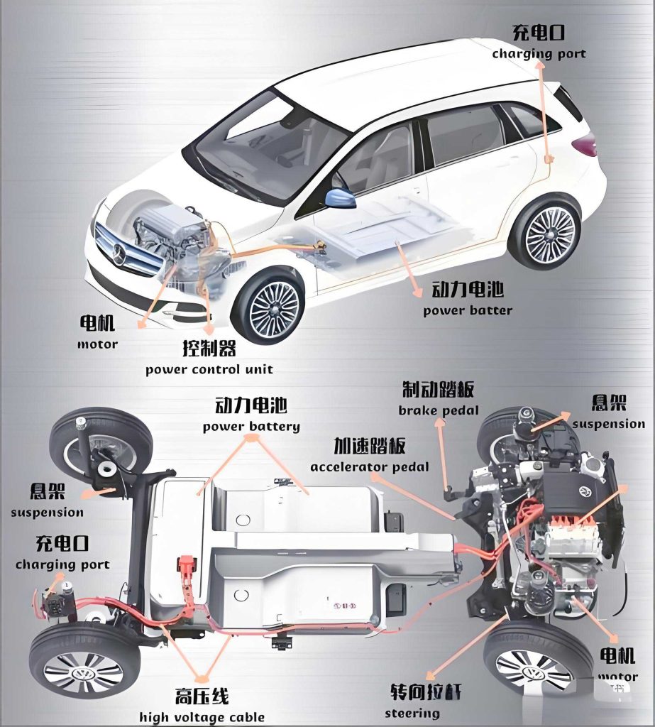
Traditional approaches to handle speed sensor faults often involve hardware redundancy, which increases cost and complexity. Model-based software solutions, such as observers, offer a more economical and elegant alternative. These observers estimate the motor speed using readily available electrical measurements (currents and voltages), effectively acting as a “virtual sensor.” Several observer-based techniques have been explored for fault-tolerant control in electric drives. Sliding mode observers (SMOs) are popular due to their inherent robustness to parameter variations and disturbances. An over-torque sliding mode observer variant has been proposed to enhance fault robustness and reduce chattering. Other methods combine higher-order SMOs with intelligent control like fuzzy logic for multiphase motor systems. While these methods provide fault tolerance, there remains room for improvement in terms of dynamic response speed, torque ripple suppression during fault operation, and the overall smoothness of the control transition, which directly impacts the driving experience of a battery electric car.
This paper presents a novel robust fault-tolerant control scheme for the motor drive system of a battery electric car, specifically targeting speed sensor failures. The core of the scheme is a cooperative observer designed to provide precise and robust estimation of the wheel motor speed when the physical sensor fails. The proposed strategy ensures seamless control reconfiguration, maintaining performance and stability. The paper is structured as follows: First, the mathematical models of the battery electric car and its six-phase permanent magnet synchronous motor (PMSM) drive are established. Subsequently, the design of the cooperative controller and the cooperative observer is detailed, followed by the description of the fault diagnosis and control reconfiguration logic. Finally, the effectiveness and superiority of the proposed scheme are demonstrated and compared against an over-torque sliding mode observer method through comprehensive hardware-in-the-loop (HIL) experiments.
System Modeling of the Battery Electric Car and Drive
1. Vehicle Dynamics Model
The longitudinal dynamics of a battery electric car are governed by the balance of forces acting upon it. The total tractive power required at the wheels to propel the vehicle is given by the product of the total force and the vehicle velocity. The forces include rolling resistance, gravitational force due to grade, aerodynamic drag, and the force required for acceleration.
$$P_{ev} = F_{total} \cdot V_{ev}$$
$$F_{total} = F_{wheel} + F_{gr} + F_{aero} + F_{acc}$$
Where $P_{ev}$ is the total drive power, $V_{ev}$ is the vehicle speed, $F_{wheel}$ is the wheel friction force, $F_{gr}$ is the force due to gravity on a slope, $F_{aero}$ is the aerodynamic drag force, and $F_{acc}$ is the inertial force for acceleration. These forces can be expanded as:
$$F_{wheel} = \mu_{roll} \cdot m_{ev} \cdot g \cdot \cos(\theta)$$
$$F_{gr} = m_{ev} \cdot g \cdot \sin(\theta)$$
$$F_{aero} = \frac{1}{2} \cdot \rho_{air} \cdot C_d \cdot A_f \cdot V_{ev}^2$$
$$F_{acc} = m_{ev} \cdot \frac{dV_{ev}}{dt}$$
To evaluate the performance of the battery electric car and its control system under realistic conditions, the ARTEMIS driving cycle is employed. This cycle provides standardized urban and road driving speed profiles. The key vehicle parameters used in this study are summarized in Table 1.
| Parameter | Symbol | Value |
|---|---|---|
| Vehicle Mass | $m_{ev}$ | 820 kg |
| Wheel Radius | $r_{wheel}$ | 0.33 m |
| Rolling Resistance Coefficient (Static) | $\mu_{roll,static}$ | 0.008 |
| Rolling Resistance Coefficient (Dynamic) | $\mu_{roll,dynamic}$ | $1.6 \times 10^{-6}$ s/m |
| Aerodynamic Drag Coefficient | $C_d$ | 0.3 |
| Frontal Area | $A_f$ | 1.8 m² |
| Air Density | $\rho_{air}$ | 1.2 kg/m³ |
| Gravitational Acceleration | $g$ | 9.8 m/s² |
| Road Grade | $\theta$ | 2.5% |
2. Six-Phase PMSM Drive Model
The propulsion system for the battery electric car in this study is a six-phase PMSM, chosen for its higher power density and inherent fault-tolerant capabilities compared to three-phase motors. It can be modeled as two sets of three-phase windings displaced by 30 electrical degrees. The mathematical model in the rotating d-q reference frame for the two three-phase sets (denoted by subscripts 1 and 2) is given below. The model assumes symmetric windings and negligible mutual coupling between the two sets.
Voltage Equations:
$$
\begin{aligned}
\frac{di_{d1}}{dt} &= \frac{1}{L_d} \left( V_{d1} – R_s i_{d1} + \omega_e L_q i_{q1} \right) \\
\frac{di_{q1}}{dt} &= \frac{1}{L_q} \left( V_{q1} – R_s i_{q1} – \omega_e L_d i_{d1} – \omega_e \psi_f \right) \\
\frac{di_{d2}}{dt} &= \frac{1}{L_d} \left( V_{d2} – R_s i_{d2} + \omega_e L_q i_{q2} \right) \\
\frac{di_{q2}}{dt} &= \frac{1}{L_q} \left( V_{q2} – R_s i_{q2} – \omega_e L_d i_{d2} – \omega_e \psi_f \right)
\end{aligned}
$$
Where $i_d$, $i_q$, $V_d$, $V_q$ are the d- and q-axis currents and voltages, $R_s$ is the stator resistance, $L_d$ and $L_q$ are the d- and q-axis inductances, $\psi_f$ is the permanent magnet flux linkage, and $\omega_e$ is the electrical angular velocity.
Electromechanical Relation:
The electrical speed is related to the mechanical rotor speed $\omega_r$ by the number of pole pairs $P$:
$$ \omega_e = \frac{P}{2} \cdot \omega_r $$
Torque and Motion Equation:
The total electromagnetic torque $T_e$ produced by the six-phase motor is the sum of the torques from both three-phase sets. For a non-salient PMSM ($L_d = L_q$), it simplifies to:
$$ T_e = \frac{3P}{2} \psi_f (i_{q1} + i_{q2}) $$
The mechanical motion of the motor is described by:
$$ J \frac{d\omega_r}{dt} = T_e – B \omega_r – T_L $$
Where $J$ is the total moment of inertia, $B$ is the viscous friction coefficient, and $T_L$ is the load torque reflecting the vehicle’s road load. The parameters of the motor drive system are listed in Table 2.
| Parameter | Symbol | Value |
|---|---|---|
| Stator Resistance | $R_s$ | 1.9 Ω |
| d-axis Inductance | $L_d$ | 0.835 mH |
| q-axis Inductance | $L_q$ | 0.835 mH |
| Number of Pole Pairs | $P$ | 4 |
| Permanent Magnet Flux | $\psi_f$ | 0.353 Wb |
| Total Inertia | $J$ | 0.015 kg·m² |
| Viscous Friction Coefficient | $B$ | 0.0954 N·m·s/rad |
| DC Bus Voltage | $V_{dc}$ | 800 V |
Proposed Fault-Tolerant Control Scheme Based on Cooperative Observer
The overarching goal is to maintain precise speed control of the battery electric car’s motor even when the speed sensor fails. The proposed architecture seamlessly integrates a cooperative controller for normal operation with a cooperative observer that acts as a virtual sensor during faults.
1. Cooperative Controller Design for Speed Regulation
The cooperative control theory provides a systematic way to design controllers by defining macroscopic variables, called manifolds, that encapsulate the desired dynamic behavior of the system. For speed control of the six-phase PMSM in the battery electric car, a first-order manifold $\psi$ is defined as the weighted combination of the speed error and its integral:
$$ \psi = \omega_{ref} – \omega_{act} + K_2 \int (\omega_{ref} – \omega_{act}) \, dt $$
or, equivalently, with the speed error $\epsilon = \omega_{ref} – \omega_{act}$:
$$ \psi = \epsilon + K_2 \int \epsilon \, dt $$
Here, $\omega_{ref}$ is the reference speed command (derived from the driver’s input and vehicle control unit), $\omega_{act}$ is the actual measured/estimated motor speed, and $K_2$ is a controller gain. The fundamental law of cooperative control dictates that the manifold must evolve according to a prescribed stable dynamics, typically a first-order decay:
$$ T_c \dot{\psi} + \psi = 0 $$
where $T_c > 0$ is a design parameter defining the convergence rate of the manifold to zero.
Substituting the expression for $\psi$ and its derivative into the cooperative law yields:
$$ T_c (\dot{\epsilon} + K_2 \epsilon) + (\epsilon + K_2 \int \epsilon \, dt) = 0 $$
Replacing $\dot{\epsilon} = \dot{\omega}_{ref} – \dot{\omega}_{act}$ and $\dot{\omega}_{act}$ from the mechanical motion equation $J \dot{\omega}_{act} = T_e – B\omega_{act} – T_L$, and assuming a constant reference speed ($\dot{\omega}_{ref}=0$), we can solve for the required electromagnetic torque $T_e^*$:
$$ T_e^* = J \left[ -\frac{1}{T_c} \epsilon – \left(K_2 + \frac{1}{T_c}\right) \int \epsilon \, dt \right] + B \omega_{act} + T_L $$
For implementation, let $K_1 = 1/T_c$. The final control law for the q-axis current reference $i_q^*$, which generates the desired torque, is derived as:
$$ i_q^* = \frac{2}{3P \psi_f} \left[ J\left( K_1 \epsilon + (K_1 K_2) \int \epsilon \, dt \right) + B \omega_{act} + T_L \right] $$
This $i_q^*$ is then used as the input to the inner-loop current controllers (e.g., PI regulators in the d-q frame) which generate the voltage commands for the inverter driving the battery electric car’s motor.
2. Cooperative Observer for Speed Sensor Fault Tolerance
When the speed sensor fails, the measured $\omega_{act}$ becomes unreliable. The cooperative observer is designed to estimate the motor speed solely from the measured phase currents and applied voltages. The process involves estimating the back-electromotive force (back-EMF) in the stationary $\alpha\beta$ reference frame, from which the rotor speed and position can be extracted.
The voltage equation in the $\alpha\beta$ frame for one three-phase set of the PMSM is:
$$ \mathbf{V}_{\alpha\beta} = R_s \mathbf{i}_{\alpha\beta} + L_s \frac{d}{dt}\mathbf{i}_{\alpha\beta} + \mathbf{e}_{\alpha\beta} $$
where $\mathbf{e}_{\alpha\beta} = [e_\alpha, e_\beta]^T$ is the back-EMF vector containing information about the rotor position $\theta_e$ and speed $\omega_e$: $e_\alpha = -\omega_e \psi_f \sin(\theta_e)$, $e_\beta = \omega_e \psi_f \cos(\theta_e)$.
The cooperative observer design follows a similar manifold approach. We define two manifolds, one for each axis ($\alpha$ and $\beta$), based on the current estimation error $\tilde{\mathbf{i}}_{\alpha\beta} = \mathbf{i}_{\alpha\beta} – \hat{\mathbf{i}}_{\alpha\beta}$, where $\hat{\mathbf{i}}_{\alpha\beta}$ is the observed current.
$$
\begin{aligned}
\psi_{\alpha} &= k_1 \tilde{i}_\alpha + k_2 \int \tilde{i}_\alpha \, dt \\
\psi_{\beta} &= k_3 \tilde{i}_\beta + k_4 \int \tilde{i}_\beta \, dt
\end{aligned}
$$
To ensure isotropic behavior, we set $k_1 = k_3$ and $k_2 = k_4$. Applying the cooperative law $T_o \dot{\psi} + \psi = 0$ to each manifold, we can derive the dynamics for the current observer. The structure of the observer is chosen to mimic the plant dynamics plus a correction term based on the manifold. The resulting equations for the estimated back-EMF components $\hat{e}_\alpha$ and $\hat{e}_\beta$ emerge as part of the observer correction signal. After derivation, the estimation law can be expressed as:
$$
\begin{aligned}
\hat{e}_\alpha &= \Gamma \left( \tilde{i}_\alpha + \frac{1}{k_1 T_o} \int \tilde{i}_\alpha \, dt \right) \\
\hat{e}_\beta &= \Gamma \left( \tilde{i}_\beta + \frac{1}{k_1 T_o} \int \tilde{i}_\beta \, dt \right)
\end{aligned}
$$
where $\Gamma$ is a gain that depends on $k_1$, $T_o$, and the machine parameters $R_s$ and $L_s$. This formulation shows that the estimated back-EMF is a cooperative function of the current error and its integral, forcing the error to converge smoothly according to the time constant $T_o$.
Finally, the rotor speed estimate $\hat{\omega}_r$ and position estimate $\hat{\theta}_e$ are calculated from the estimated back-EMF:
$$
\begin{aligned}
\hat{\omega}_e &= \frac{\sqrt{\hat{e}_\alpha^2 + \hat{e}_\beta^2}}{\psi_f} \\
\hat{\omega}_r &= \frac{2}{P} \hat{\omega}_e \\
\hat{\theta}_e &= \arctan2(-\hat{e}_\alpha, \hat{e}_\beta)
\end{aligned}
$$
This $\hat{\omega}_r$ serves as the virtual speed sensor signal for the battery electric car’s drive controller.
3. Fault Diagnosis and Control Reconfiguration Logic
A key element of the fault-tolerant control scheme for the battery electric car is the automatic detection of the speed sensor fault and the subsequent reconfiguration of the control loop. The fault is diagnosed by comparing the speed from the physical sensor $\omega_r$ with the estimate from the always-running cooperative observer $\hat{\omega}_r$.
A residual signal $R(t)$ is generated:
$$ R(t) = | \omega_r(t) – \hat{\omega}_r(t) | $$
Under normal operation, the observer is tuned to track the true speed closely, so the residual $R(t)$ is very small, consisting only of estimation errors and noise. When a sensor fault occurs (e.g., a bias, gain error, or complete signal loss), the measured $\omega_r$ deviates significantly from the true value, while the observer estimate $\hat{\omega}_r$ remains accurate as it is based on healthy electrical signals. Consequently, the residual $R(t)$ exceeds a pre-defined threshold $R_{th}$.
The fault detection flag $F$ is generated using a simple logic:
$$
F = \begin{cases}
1 & \text{if } R(t) > R_{th} \text{ for a duration } t > t_{debounce} \\
0 & \text{otherwise}
\end{cases}
$$
A debounce time $t_{debounce}$ is used to prevent false alarms due to transients or noise spikes. Once $F$ is set to 1, the fault management system triggers the control reconfiguration. The switch in the feedback path changes from the faulty physical sensor signal $\omega_r$ to the robust estimate $\hat{\omega}_r$ provided by the cooperative observer. This transition is bumpless due to the observer’s continuous operation and accurate tracking. The control law of the cooperative controller now uses $\hat{\omega}_r$ as $\omega_{act}$, ensuring uninterrupted and stable operation of the battery electric car’s motor drive.
Hardware-in-the-Loop Validation and Analysis
The proposed robust fault-tolerant control scheme for the battery electric car drive system was rigorously validated using a hardware-in-the-loop test platform. The setup consisted of a real-time simulator (e.g., OPAL-RT) running the detailed models of the six-phase PMSM, the inverter, and the vehicle dynamics, while the control algorithms (cooperative controller, cooperative observer, fault diagnosis) were executed on a dedicated microcontroller unit (MCU) board interfacing with the simulator.
1. Motor Drive System Performance Under Sensor Fault
First, the performance of the motor drive alone was tested. The reference speed was set to 50 rad/s, stepped up to 100 rad/s at t=0.5s, and back to 50 rad/s at t=1.0s. A load torque disturbance was applied at t=1.5s. Crucially, a complete failure of the speed sensor was simulated at t=0.35s. The performance of the proposed cooperative observer-based FTC was compared against the benchmark over-torque sliding mode observer (OTSMO) based FTC.
The results demonstrated that both FTC strategies successfully managed the sensor fault, preventing system shutdown. However, distinct performance differences were observed, as quantified in Table 3.
| Metric | Proposed Cooperative Observer FTC | OTSMO-based FTC |
|---|---|---|
| Fault Detection & Reconfiguration Time | ~14 ms | ~18 ms |
| Speed Tracking Error (RMS after fault) | 0.45 rad/s | 0.68 rad/s |
| Torque Ripple (Peak-to-Peak) during fault operation | 1.2 Nm | 2.8 Nm |
| Current THD after reconfiguration | 2.1% | 3.9% |
| Speed Overshoot at t=0.5s step (using estimated speed) | 3.5% | 7.2% |
The proposed scheme showed a faster reconfiguration time, lower steady-state tracking error, and significantly reduced torque and current ripple. The smoother manifold-based dynamics of the cooperative observer resulted in less chattering, translating to better quality of torque delivery, which is crucial for the driving feel of a battery electric car. The speed response during the step command at t=0.5s, executed solely based on the observer estimate after the fault, was quicker and with less overshoot compared to the OTSMO method.
2. Integrated Vehicle-Level Validation on Driving Cycle
To assess the holistic performance in a realistic scenario for a battery electric car, the integrated system (vehicle model + motor + FTC) was tested under the ARTEMIS driving cycle. The speed sensor fault was injected at t=16 seconds during an acceleration phase.
The vehicle speed tracking performance is shown in Figure X. The fault was detected within approximately 10 ms, and the control loop seamlessly reconfigured to use the cooperative observer’s estimate. The battery electric car continued to follow the demanded speed profile accurately, with no noticeable deviation or jerk perceptible in the speed trace. The transitions during acceleration and deceleration phases remained smooth.
The corresponding motor torque and power output are shown in Figure Y. The torque demand from the vehicle controller was met faithfully by the fault-tolerant drive system. The power output profile remained consistent with the demands of the driving cycle. Key performance metrics for the battery electric car during this fault scenario are summarized in Table 4.
| Metric | Value |
|---|---|
| Fault Injection Time | t = 16.0 s |
| Fault Detection & Reconfiguration Delay | 10.5 ms |
| Max Absolute Speed Error Post-Fault (vs. Cycle) | 0.32 km/h |
| RMS Speed Tracking Error Post-Fault | 0.11 km/h |
| Peak Drivetrain Torque Disturbance during Reconfiguration | 15 Nm |
| Vehicle Stopping Distance (simulated emergency stop post-fault) | Within 2% of nominal (no-fault) distance |
The results confirm that the proposed robust fault-tolerant control scheme effectively manages a critical speed sensor failure in the battery electric car’s drive system. The vehicle maintains its intended speed trajectory, drivability is preserved, and safety-critical maneuvers like braking remain effective, all without any intervention from the driver.
Conclusion
This paper presented a comprehensive robust fault-tolerant control solution for the motor drive system of a battery electric car, specifically addressing the critical issue of speed sensor failure. The scheme leverages the synergistic design of a cooperative controller for performance and a cooperative observer for fault tolerance. The cooperative controller ensures dynamic speed tracking with prescribed dynamics, while the cooperative observer provides a precise, chattering-free estimate of the motor speed to be used as a virtual sensor upon physical sensor failure. The integrated fault diagnosis logic enables fast and reliable detection and automatic, bumpless control reconfiguration.
Through detailed hardware-in-the-loop testing, the proposed scheme demonstrated superior performance compared to a benchmark over-torque sliding mode observer method. It exhibited faster dynamic response, lower speed tracking error, and significantly reduced torque ripple during fault operation, contributing to a smoother and more reliable driving experience for the battery electric car. Furthermore, validation under a standard driving cycle confirmed the scheme’s effectiveness at the full vehicle level, ensuring continued safe and controlled operation even with a faulty speed sensor. The proposed approach offers a viable and high-performance solution to enhance the reliability and safety of battery electric cars, paving the way for more robust automotive propulsion systems.