
In the context of the global “dual carbon” strategy, the new energy vehicle industry has developed rapidly due to its advantages of quietness, high efficiency, and zero pollution emissions. As the core energy storage component of new energy vehicles, the power battery pack directly determines the vehicle’s cruising range, safety, and service life. Lithium-ion batteries, with their high energy density, low self-discharge rate, and long cycle life, have become the dominant power source for modern electric vehicles. However, these batteries generate significant heat during operation due to internal electrochemical reactions and ohmic losses. If this heat is not effectively managed, it can lead to performance degradation, accelerated aging, and in extreme cases, thermal runaway—a catastrophic event that poses severe safety risks. Furthermore, the battery pack housing must withstand various mechanical loads during vehicle operation, including acceleration shocks, vibrations, and potential impacts. Therefore, the design of an efficient thermal management system and a structurally robust battery pack enclosure are two critical aspects that determine the overall performance and safety of the vehicle. This article presents a comprehensive investigation into the design and optimization of a power battery pack for a new energy vehicle, focusing on both the liquid cooling thermal management system and the structural integrity of the battery pack housing.
Thermal Characteristics of Lithium-Ion Batteries and CFD Methodology
To design an effective thermal management system for the electric vehicle battery, it is essential to first understand the fundamental working principles and heat generation mechanisms of lithium-ion batteries. A lithium-ion battery consists of positive and negative electrodes, an electrolyte, current collectors, and a separator. The positive electrode materials commonly include lithium iron phosphate (LiFePO₄), lithium nickel manganese cobalt oxide (NMC), and lithium cobalt oxide (LiCoO₂). Among these, NMC and LiFePO₄ are the most widely used in electric vehicle battery packs due to their balanced performance in terms of energy density, safety, and cost. The negative electrode is typically made of graphite, which offers excellent lithium-ion intercalation capacity and stability. The electrolyte, usually a lithium salt such as LiPF₆ dissolved in organic solvents, facilitates ion transport between the electrodes.
The working principle of a lithium-ion battery relies on the reversible intercalation and deintercalation of lithium ions between the positive and negative electrodes. During charging, lithium ions are extracted from the positive electrode and inserted into the negative electrode through the electrolyte, while electrons flow through the external circuit. This process is reversed during discharge. The electrochemical reactions can be expressed as follows:
Positive electrode reaction:
$$ \mathrm{LiM_yO_z} \xrightleftharpoons{\text{charge/discharge}} \mathrm{Li_{x}M_yO_z} + x\mathrm{Li^+} + x e^- $$
Negative electrode reaction:
$$ \mathrm{C} + x\mathrm{Li^+} + x e^- \xrightleftharpoons{\text{charge/discharge}} \mathrm{Li_xC} $$
Overall cell reaction:
$$ \mathrm{LiM_yO_z} + \mathrm{C} \xrightleftharpoons{\text{charge/discharge}} \mathrm{Li_xM_yO_z} + \mathrm{Li_{1-x}C} $$
During operation, the total heat generated within a battery, denoted as \( Q_{total} \), consists of four components: electrochemical reaction heat \( Q_r \), polarization heat \( Q_p \), ohmic heat \( Q_j \), and side reaction heat \( Q_s \). The electrochemical reaction heat is a reversible phenomenon associated with entropy changes during the intercalation/deintercalation processes. Polarization heat arises from the deviation from equilibrium potential during current flow, while ohmic heat is produced by the internal resistance of the battery materials. Side reaction heat, which is typically negligible under normal operating conditions, becomes significant only during thermal runaway events. The total heat generation can be accurately described by the Bernadi heat generation rate model:
$$ Q_{total} = Q_r + Q_p + Q_j = I^2 R + IT \frac{\partial U_{ocv}}{\partial T} $$
where \( I \) is the discharge current, \( R \) is the internal resistance, \( U_{ocv} \) is the open-circuit voltage, and \( T \) is the battery temperature. This model provides a theoretical foundation for predicting battery temperature rise under various operating conditions.
Heat transfer within a battery pack occurs primarily through two mechanisms: heat conduction and heat convection. Heat conduction, governed by Fourier’s law, transfers heat from the battery core to its surface:
$$ \Phi = -\lambda A \frac{dt}{dx} $$
where \( \lambda \) is the thermal conductivity, \( A \) is the contact area, and \( \frac{dt}{dx} \) is the temperature gradient. Heat convection, described by Newton’s law of cooling, dissipates heat from the battery surface to the surrounding medium:
$$ \Phi = hA(t_w – t_f) $$
where \( h \) is the convective heat transfer coefficient, \( t_w \) is the wall temperature, and \( t_f \) is the fluid temperature. For forced convection in channels, the Nusselt number can be correlated using the Gnielinski equation:
$$ Nu = \frac{(f/8)(Re – 1000)Pr}{1 + 12.7\sqrt{f/8}(Pr^{2/3} – 1)} \left[ 1 + \left( \frac{d}{l} \right)^{2/3} \right] $$
with the Darcy friction factor given by the Konakov formula:
$$ f = (1.8 \log_{10} Re – 1.5)^{-2} $$
and the Reynolds number:
$$ Re = \frac{\rho u d}{\mu} $$
Computational Fluid Dynamics (CFD) serves as a powerful tool for simulating these heat transfer phenomena. The simulation process involves three main stages: pre-processing (geometry creation and mesh generation), solving (setting boundary conditions and running the solver), and post-processing (visualizing and analyzing results). The governing equations for fluid flow and heat transfer in CFD simulations are the conservation equations of mass, momentum, and energy. For incompressible coolants used in electric vehicle battery thermal management systems:
Continuity equation:
$$ \nabla \cdot \mathbf{v} = 0 $$
Momentum equation:
$$ \rho \frac{\partial \mathbf{v}}{\partial t} + \rho (\mathbf{v} \cdot \nabla) \mathbf{v} = -\nabla p + \mu \nabla^2 \mathbf{v} + \rho g $$
Energy equation:
$$ \rho c_p \frac{\partial T}{\partial t} + \rho c_p (\mathbf{v} \cdot \nabla) T = \lambda \nabla^2 T $$
Battery Pack Design and Single Cell Thermal Analysis
Battery Pack Sizing and Configuration
The first step in the design process of the electric vehicle battery was to determine the required battery capacity based on the target driving range. Referring to the NEDC (New European Driving Cycle) driving cycle, I calculated the energy consumption for both constant-speed and constant-acceleration phases. The NEDC cycle consists of four repeated urban driving cycles followed by one extra-urban driving cycle, totaling approximately 11 km with an average speed of 33.6 km/h. For a target cruising range of 200 km, the total energy consumption was calculated by considering the forces acting on the vehicle: rolling resistance \( F_f \), aerodynamic drag \( F_w \), and acceleration resistance \( F_a \).
$$ F_f = mgf \cos \alpha $$
$$ F_w = \frac{1}{2} \rho_{air} C_D A v^2 $$
$$ F_a = \delta m \frac{dv}{dt} $$
Using the vehicle parameters listed below, I calculated the energy consumption for each phase of the driving cycle.
| Parameter | Symbol | Value |
|---|---|---|
| Test mass | m | 1700 kg |
| Rolling resistance coefficient | f | 0.008 |
| Drag coefficient | C_D | 0.36 |
| Frontal area | A | 2.47 m² |
| Rotational mass conversion factor | δ | 1.06 |
| Transmission efficiency | η₁ | 0.9 |
| Depth of discharge | η₂ | 0.9 |
| Discharge efficiency | η₃ | 0.95 |
| Ancillary power consumption rate | η₄ | 0.1 |
The energy consumption for constant-speed phases was calculated using:
$$ W_f = \frac{mgfv t}{3.6 \eta_1} $$
$$ W_w = \frac{0.5 \rho C_D A v^3 t}{3.6 \eta_1} $$
The energy consumption for acceleration phases incorporated the inertial force:
$$ W_a = \frac{\delta ma (v_0 t + 0.5 a t^2)}{3.6 \eta_1} $$
Table 2 summarizes the energy consumption for constant-speed driving phases, and Table 3 for acceleration phases. The total energy required to complete the target range was calculated to be approximately 40.5 kWh.
| Speed (km/h) | Duration (s) | Rolling resistance energy (J) | Aerodynamic drag energy (J) |
|---|---|---|---|
| 15 | 32 | 19,745.19 | 108.13 |
| 32 | 96 | 126,369.19 | 3,149.64 |
| 50 | 117 | 240,644.44 | 14,643.16 |
| 35 | 60 | 86,385.19 | 2,575.70 |
| 70 | 50 | 143,975.31 | 4,769.81 |
| 100 | 30 | 123,407.41 | 8,343.68 |
| 120 | 10 | 49,362.96 | 4,805.96 |
The total energy consumption from constant-speed segments was approximately 0.23 kWh, while the acceleration segments contributed approximately 1.46 kWh, as shown in the following table.
| Speed range (km/h) | Acceleration (m/s²) | Duration (s) | Cycles | Rolling energy (J) | Aerodynamic energy (J) | Acceleration energy (J) |
|---|---|---|---|---|---|---|
| 0-15 | 0.83 | 5 | 8 | 1,543.83 | 4.23 | 17,408.22 |
| 15-32 | 0.81 | 11 | 8 | 7,239.90 | 90.22 | 79,100.14 |
| 0-50 | 0.56 | 25 | 4 | 25,709.88 | 782.22 | 193,115.57 |
| 50-35 | 0.52 | 8 | 4 | 13,985.51 | 453.45 | 98,563.09 |
| 0-35 | 0.97 | 10 | 4 | 7,198.77 | 107.32 | 94,626.63 |
| 0-70 | 0.47 | 41 | 1 | 59,029.88 | 3,520.12 | 378,506.52 |
| 70-50 | 0.56 | 10 | 2 | 24,679.01 | 1,662.54 | 185,187.04 |
| 0-4.17 | 0.83 | 5 | 1 | 122,373.25 | 22,189.28 | 394,252.37 |
| 0-32 | 0.81 | 11 | 1 | 90,497.12 | 26,871.44 | 339,537.35 |
| 0-120 | 0.56 | 25 | 1 | 83,917.04 | 14,706.24 | 1,112,345.68 |
The minimum required battery energy was calculated as:
$$ E_{total} = \frac{(W + W’) \times ER}{\eta_2 \eta_3 (1 – \eta_4) \times D} $$
which yielded approximately 39.53 kWh. To provide sufficient margin, I selected a battery pack with 40.5 kWh total energy, consisting of 96 prismatic NMC lithium-ion cells connected in series. The battery pack voltage was calculated as 355.2 V (96 cells × 3.7 V), which falls within the typical motor operating voltage range of 250-420 V.
To determine the maximum discharge rate of the electric vehicle battery, I calculated the power requirements for three key performance metrics: maximum speed, maximum gradeability, and acceleration performance. The power required at maximum speed (200 km/h) was:
$$ P_1 = \frac{v_1}{3600 \eta_1} \left( mgf + \frac{C_D A v_1^2}{21.15} \right) = 112.04 \text{ kW} $$
The power required for maximum gradeability (16.7° at 30 km/h) was:
$$ P_2 = \frac{v_2}{3600 \eta_1} \left( mgf \cos \alpha + mg \sin \alpha + \frac{C_D A v_2^2}{21.15} \right) = 45.86 \text{ kW} $$
The power required for 0-100 km/h acceleration in 8 seconds was:
$$ P_3 = \frac{v_3}{3600 \eta_1} \left( \delta m \frac{v_3}{t} + mgf + \frac{C_D A v_3^2}{21.15} \right) = 113.95 \text{ kW} $$
From these calculations, the maximum power demand was determined to be 113.95 kW, requiring a maximum discharge rate of 3C from the battery pack. Table 5 summarizes the specifications of the selected single cell.
| Parameter | Value |
|---|---|
| Rated capacity | 114 Ah |
| Internal resistance | 0.4 mΩ |
| Density | 2219 kg/m³ |
| Specific heat capacity | 1000 J/(kg·K) |
| Thermal conductivity (x, y, z) | 2.5, 12, 12 W/(m·K) |
| Nominal voltage | 3.7 V |
The battery pack model comprised three modules, each containing 32 cells. Thermal insulation plates made of phenolic resin were placed between modules to reduce heat transfer between adjacent cells, ensuring thermal uniformity within the electric vehicle battery pack. The bottom of the battery pack was designed to accommodate a liquid cooling plate, as the thermal conductivity in the vertical direction of the battery is significantly higher than in the horizontal direction.
Single Cell Thermal Simulation
Using the Bernadi heat generation model, I calculated the heat source power for different discharge rates: 5.2 W at 1C, 20.8 W at 2C, and 46.8 W at 3C. The corresponding discharge times were 3600 s, 1800 s, and 1200 s, respectively. The grid independence study was conducted using six different mesh densities, ranging from 313,557 to 1,827,666 elements. The simulation results, presented in Table 6, demonstrated that the maximum temperature variation between the coarsest and finest meshes was only 0.02°C, indicating acceptable grid convergence.
| Parameter | Scheme 1 | Scheme 2 | Scheme 3 | Scheme 4 | Scheme 5 | Scheme 6 |
|---|---|---|---|---|---|---|
| Mesh size setting | 10:30 | 7:30 | 5:30 | 4:30 | 3:30 | 2:30 |
| Element count | 313,557 | 593,633 | 1,044,646 | 1,495,842 | 1,627,727 | 1,827,666 |
| Average orthogonal quality | 0.75 | 0.85 | 0.87 | 0.89 | 0.89 | 0.89 |
| Maximum temperature (°C) | 30.26 | 30.25 | 30.25 | 30.28 | 30.28 | 30.28 |
| Flow resistance (Pa) | 858.08 | 794.12 | 816.25 | 833.85 | 807.20 | 811.32 |
Based on the grid independence study, I selected Scheme 5 with 1,627,727 elements for subsequent simulations, balancing accuracy and computational efficiency. Table 7 presents the simulation results of the single cell thermal analysis at different discharge rates.
| Parameter | 1C | 2C | 3C |
|---|---|---|---|
| Maximum temperature (°C) | 33.03 | 43.08 | 53.41 |
| Temperature rise (°C) | 8.03 | 18.08 | 28.41 |
The simulation results revealed that the temperature distribution on the battery surface was not uniform. The corners and edges showed lower temperatures due to natural convection with the surrounding air, while the center of the battery face exhibited higher temperatures. The top and side surfaces maintained higher temperatures than the front face, which had a larger contact area with air. This temperature distribution pattern correlates with the internal structure of the battery, where the stacking of electrode layers creates anisotropic thermal conductivity. The internal temperature was found to be higher than the external surface temperature, indicating heat accumulation within the battery core. This observation confirms the necessity of a liquid cooling plate placed at the bottom of the battery pack for the electric vehicle battery, as the vertical thermal conductivity is significantly higher than the horizontal direction.
Liquid Cooling System Design and Optimization
Liquid Cold Plate Concept Design
Based on a comprehensive review of thermal management technologies, I selected the liquid cooling plate heat exchange method for the electric vehicle battery thermal management system due to its high cooling efficiency, simple structure, and cost-effectiveness. Table 8 lists the material properties used in the simulations.
| Component | Material | Density (kg/m³) | Specific heat (J/(kg·K)) | Thermal conductivity (W/(m·K)) |
|---|---|---|---|---|
| Insulation plate | Phenolic resin | 1800 | 1650 | 0.15 |
| Cold plate | Aluminum alloy | 2700 | 900 | 247 |
| Coolant | Water | 997.05 | 4200 | 0.607 |
Figure 4 illustrates two liquid cold plate designs: (a) a parallel flow channel design with a serpentine arrangement, and (b) a traditional single serpentine flow channel. In the parallel design, the coolant enters a distribution region, splits into multiple parallel channels, and then merges in a collection region before exiting. This design reduces the coolant velocity, extends the residence time, and enhances heat transfer. The serpentine design has a single flow channel that winds through the plate, maintaining higher coolant velocity throughout.
Both designs incorporate inlet and outlet ports with a diameter of 12 mm, channel width of 25 mm, and plate thickness of 6 mm. Table 9 presents the key simulation results under identical operating conditions (1C discharge rate, 0.05 kg/s coolant flow rate, 25°C initial temperature).
| Parameter | Parallel flow channel | Single serpentine channel |
|---|---|---|
| Maximum temperature (°C) | 30.28 | 29.92 |
| Temperature difference (°C) | 2.16 | 2.45 |
| Flow resistance (Pa) | 807.20 | 6,878.71 |
Although the serpentine design achieved a slightly lower maximum temperature (29.92°C vs. 30.28°C) due to higher coolant velocity in the single channel, the flow resistance was dramatically higher (6,878.71 Pa vs. 807.20 Pa). The parallel flow design was selected for further analysis because of its significantly lower pressure drop, which reduces the pumping power requirement and improves energy efficiency of the thermal management system.
Coolant Selection
The selection of an appropriate coolant medium is crucial for the thermal performance of the electric vehicle battery cooling system. I evaluated four coolant candidates: pure water and ethylene glycol (EG) solutions at 30wt%, 50wt%, and 70wt% concentrations. The thermophysical properties of these coolants are summarized in Table 10.
| Property | Water | 30wt% EG | 50wt% EG | 70wt% EG |
|---|---|---|---|---|
| Density (kg/m³) | 997.3 | 1012.4 | 1034.4 | 1065.3 |
| Specific heat (J/(kg·K)) | 4190 | 3572.1 | 3212.2 | 2852.1 |
| Dynamic viscosity (mPa·s) | 0.80 | 1.6431 | 2.8454 | 5.0962 |
| Thermal conductivity (W/(m·K)) | 0.607 | 0.4424 | 0.3610 | 0.3011 |
| Freezing point (°C) | 0 | -14.1 | -33.8 | < -50 |
The simulation results, shown in Figure 5, revealed that the maximum battery temperature increases with increasing EG concentration. This is attributed to the combined effects of reduced specific heat capacity and increased viscosity, which impair the convective heat transfer coefficient. However, considering the freezing point requirements for cold climate operation, pure water is unsuitable. The 50wt% EG solution provides an optimal balance between cooling performance and cold-weather operability, with a freezing point of -33.8°C.
To further enhance the cooling performance, I investigated the addition of Al₂O₃ nanoparticles to the 50wt% EG solution, creating nanofluids with mass fractions of 0.3%, 0.5%, 0.8%, and 2%. Table 11 lists properties of the nanofluids.
| Property | 0.3wt% | 0.5wt% | 0.8wt% | 2wt% |
|---|---|---|---|---|
| Density (kg/m³) | 1036.7 | 1038.2 | 1040.5 | 1049.9 |
| Specific heat (J/(kg·K)) | 3204.9 | 3200.1 | 3192.8 | 3163.5 |
| Dynamic viscosity (mPa·s) | 2.851 | 2.8547 | 2.8604 | 2.8831 |
| Thermal conductivity (W/(m·K)) | 0.3618 | 0.3624 | 0.3632 | 0.3666 |
The simulation results indicated that the addition of nanoparticles produced only marginal improvements in cooling performance (temperature reduction less than 0.1°C), while the flow resistance slightly decreased. Given the increased cost and complexity associated with nanofluids, the 50wt% EG solution was ultimately selected as the most suitable coolant for the electric vehicle battery thermal management system.
Effect of Channel Number on Cooling Performance
To optimize the parallel flow channel design, I investigated the effect of the number of channels on the cooling performance of the liquid cooling plate. Four configurations with 2, 3, 4, and 5 channels were designed, maintaining the same overall plate dimensions and channel width of 25 mm. The simulation results are presented in Table 12 and illustrated in the following figures.
| Channel number | Maximum temperature (°C) | Temperature difference (°C) | Flow resistance (Pa) |
|---|---|---|---|
| 2 channels | 32.43 | 3.5 | 2,150.36 |
| 3 channels | 31.56 | 3.2 | 1,580.24 |
| 4 channels | 31.28 | 3.0 | 1,210.85 |
| 5 channels | 30.68 | 2.6 | 962.88 |
The analysis of the simulation results revealed that increasing the number of channels from 2 to 5 reduced the maximum battery temperature by 1.75°C. This improvement is primarily attributed to the increased contact area between the coolant and the plate material, which enhances the convective heat transfer according to Newton’s law of cooling. Additionally, the parallel flow configuration causes the coolant to split into multiple streams, reducing the flow velocity in each channel and consequently decreasing the flow resistance. The 5-channel design achieved the best overall performance with a maximum temperature of 30.68°C, a temperature difference of 2.6°C, and a flow resistance of 962.88 Pa.
Table 13 presents the calculated Reynolds numbers for the coolant flowing through the channels of each configuration, confirming that the flow regime remains laminar (Re < 2300) in all cases.
| Design | Channel 1 | Channel 2 | Channel 3 | Channel 4 | Channel 5 |
|---|---|---|---|---|---|
| 2 channels | 592.35 | 526.57 | – | – | – |
| 3 channels | 407.87 | 397.46 | 310.65 | – | – |
| 4 channels | 313.73 | 318.73 | 283.02 | 206.47 | – |
| 5 channels | 261.63 | 265.69 | 269.34 | 197.28 | 131.36 |
Effect of Channel Width on Cooling Performance
I further investigated the influence of channel width on the cooling performance by comparing four designs with channel widths of 10 mm, 15 mm, 20 mm, and 25 mm, while maintaining five channels in each configuration. The simulation results are summarized in Table 14.
| Channel width (mm) | Maximum temperature (°C) | Temperature difference (°C) | Flow resistance (Pa) |
|---|---|---|---|
| 10 | 31.48 | 3.4 | 2,054.87 |
| 15 | 31.05 | 3.1 | 1,585.63 |
| 20 | 30.82 | 2.9 | 1,220.45 |
| 25 | 30.68 | 2.6 | 962.88 |
The results indicated that wider channels provide better cooling performance due to the increased heat transfer area. Although narrower channels increase the coolant velocity (as shown in Table 15), the flow remains laminar, and the velocity increase does not compensate for the reduced contact area. The 25 mm channel width design was selected as optimal for the electric vehicle battery thermal management system.
| Channel width | Channel 1 velocity (m/s) | Channel 1 Re | Channel 5 velocity (m/s) | Channel 5 Re |
|---|---|---|---|---|
| 25 mm | 0.0742 | 261.63 | 0.0373 | 131.36 |
| 20 mm | 0.0887 | 296.58 | 0.0570 | 190.64 |
| 15 mm | 0.1158 | 362.01 | 0.0842 | 263.11 |
| 10 mm | 0.1678 | 457.43 | 0.1416 | 386.09 |
Effect of Coolant Inlet Conditions
Using the optimized liquid cold plate design, I conducted transient simulations to evaluate the cooling performance under different discharge rates and coolant inlet conditions. The boundary conditions were set with a 25°C initial temperature, and the coolant inlet temperature and flow rate were varied as parameters.
For the 2C discharge rate (1800 s discharge time, 20.8 W per cell heat generation), I evaluated coolant flow rates of 0.06, 0.08, and 0.1 kg/s. The simulation results are presented in Table 16.
| Flow rate (kg/s) | Maximum temperature (°C) | Temperature difference (°C) | Flow resistance (Pa) |
|---|---|---|---|
| 0.06 | 38.48 | 3.8 | 1,285.80 |
| 0.08 | 37.90 | 3.3 | 2,057.64 |
| 0.10 | 37.49 | 3.0 | 3,003.24 |
All three flow rates were able to maintain the maximum battery temperature below the upper limit of the recommended operating range (40°C). The minimum flow rate of 0.06 kg/s was sufficient to cool the electric vehicle battery at 2C discharge, providing a maximum temperature of 38.48°C. This flow rate was selected to minimize pumping power consumption while maintaining acceptable thermal performance.
For the 3C discharge rate (1200 s discharge time, 46.8 W per cell heat generation), I evaluated higher coolant flow rates of 0.1, 0.2, and 0.3 kg/s. Table 17 presents the simulation results.
| Flow rate (kg/s) | Maximum temperature (°C) | Temperature difference (°C) | Flow resistance (Pa) |
|---|---|---|---|
| 0.1 | 46.89 | 4.4 | 3,003.24 |
| 0.2 | 45.35 | 3.2 | 11,258.18 |
| 0.3 | 44.72 | 2.9 | 23,718.70 |
None of the flow rates were able to reduce the maximum temperature to within the recommended operating range for the electric vehicle battery. The temperature distribution cloud map revealed significant heat accumulation in the upper portion of the battery pack, as the liquid cooling plate was only placed at the bottom. Additionally, at higher flow rates, the flow trajectory analysis showed that coolant tended to recirculate in the merging regions of the parallel channels, creating flow maldistribution and substantially increasing the pressure drop.
I then investigated the effect of reducing the coolant inlet temperature while maintaining a flow rate of 0.1 kg/s. The results are presented in Table 18.
| Inlet temperature (°C) | Maximum temperature (°C) | Temperature difference (°C) |
|---|---|---|
| 20 | 44.83 | 5.3 |
| 15 | 42.52 | 6.3 |
| 10 | 41.03 | 7.9 |
Although reducing the inlet temperature effectively lowered the maximum battery temperature, it significantly worsened the temperature uniformity across the battery pack. With a 10°C inlet temperature, the temperature difference between cells reached 7.9°C, exceeding the recommended maximum of 5°C. This is because the coolant heated up substantially as it flowed through the channels, reducing its cooling capacity near the outlet side of the electric vehicle battery pack.
Double-Layer Liquid Cooling Plate Design
To address the excessive temperature rise at 3C discharge rate while maintaining temperature uniformity, I proposed a double-layer liquid cooling plate configuration. As illustrated in the model, an additional cooling plate was placed on top of the battery pack. The upper plate requires careful electrical insulation due to the presence of busbars and current collectors in that region. The insulation design uses a plastic fixture as a carrier for the busbars and ceramic insulation materials. A thermally conductive material was added between the plastic fixture and the cooling plate to overcome the low thermal conductivity of the plastic.
In this configuration, both the upper and lower cooling plates receive a coolant flow rate of 0.1 kg/s. The inlet and outlet ports on the two plates were positioned on opposite sides to minimize the temperature gradient across the electric vehicle battery pack. The simulation results showed that the double-layer design successfully reduced the maximum battery temperature at 3C discharge to 37.92°C, which is within the recommended operating range. The temperature difference between cells was reduced to 2.6°C, also satisfying the design requirement of less than 5°C.
The temperature distribution analysis revealed that the upper cooling plate performed slightly less effectively than the lower plate, with a temperature difference of approximately 1°C. This is attributed to the additional thermal resistance introduced by the plastic fixture, busbars, and ceramic insulation materials. However, the thermally conductive filler material effectively mitigated this issue, enabling sufficient heat transfer from the top of the battery pack.
Parameter Optimization of the Liquid Cooling Plate
From the simulation results at higher coolant flow rates, I observed that significant vortices form in the channel merging regions of the liquid cooling plate at elevated flow rates, leading to increased flow resistance. To address this issue, I conducted a parameter optimization study using the following methodology:
- Define design variables based on the channel gap dimensions in the merging regions
- Generate sample points using Optimal Latin Hypercube Design (OLHD)
- Build a surrogate model using the Response Surface Method (RSM)
- Optimize using the NSGA-II algorithm
The design variables were defined as X1 through X7, representing the four merging gaps and three serpentine return gaps, each ranging from 20 mm to 60 mm. The optimization objectives were the coolant flow resistance (Y1) and the coolant outlet average temperature (Y2). To reduce computational time, the liquid cooling plate was simulated with a constant heat flux applied on its top surface, approximating the heat generated by the electric vehicle battery at 1C discharge rate.
Table 19 presents the 39 design points generated by the OLHD method along with their corresponding simulation results.
| Sample | X1 (mm) | X2 (mm) | X3 (mm) | X4 (mm) | X5 (mm) | X6 (mm) | X7 (mm) | Y1 (Pa) | Y2 (°C) |
|---|---|---|---|---|---|---|---|---|---|
| 1 | 38 | 37 | 48 | 44 | 78 | 76 | 42 | 711.53 | 26.56 |
| 2 | 42 | 32 | 55 | 58 | 51 | 73 | 55 | 698.80 | 26.57 |
| 3 | 53 | 36 | 50 | 40 | 74 | 32 | 62 | 736.60 | 26.56 |
| 4 | 36 | 60 | 56 | 40 | 51 | 50 | 47 | 728.93 | 26.57 |
| 5 | 34 | 33 | 39 | 44 | 43 | 80 | 47 | 765.10 | 26.56 |
| 6 | 60 | 48 | 46 | 32 | 44 | 71 | 63 | 741.98 | 26.57 |
| 7 | 47 | 50 | 55 | 33 | 71 | 59 | 75 | 715.91 | 26.56 |
| 8 | 36 | 39 | 60 | 48 | 36 | 43 | 49 | 789.91 | 26.58 |
| 9 | 54 | 41 | 42 | 36 | 46 | 40 | 80 | 744.95 | 26.56 |
| 10 | 36 | 39 | 38 | 54 | 33 | 47 | 41 | 838.54 | 26.57 |
| 11 | 32 | 43 | 52 | 58 | 63 | 54 | 35 | 720.27 | 26.57 |
| 12 | 58 | 52 | 31 | 47 | 37 | 56 | 67 | 753.78 | 26.57 |
| 13 | 34 | 57 | 35 | 54 | 52 | 67 | 48 | 734.69 | 26.56 |
| 14 | 35 | 32 | 54 | 41 | 59 | 62 | 77 | 730.88 | 26.56 |
| 15 | 37 | 56 | 40 | 48 | 79 | 53 | 74 | 688.12 | 26.56 |
| 16 | 42 | 53 | 37 | 38 | 31 | 75 | 53 | 806.81 | 26.57 |
| 17 | 49 | 47 | 60 | 37 | 58 | 77 | 45 | 706.20 | 26.57 |
| 18 | 30 | 52 | 45 | 54 | 55 | 33 | 59 | 751.70 | 26.56 |
| 19 | 46 | 56 | 47 | 60 | 41 | 46 | 37 | 744.78 | 26.58 |
| 20 | 41 | 41 | 34 | 51 | 79 | 33 | 51 | 735.87 | 26.56 |
| 21 | 31 | 45 | 46 | 49 | 33 | 61 | 71 | 818.88 | 26.57 |
| 22 | 43 | 48 | 59 | 50 | 55 | 41 | 79 | 689.65 | 26.57 |
| 23 | 40 | 58 | 39 | 35 | 49 | 55 | 78 | 737.72 | 26.57 |
| 24 | 40 | 46 | 30 | 40 | 69 | 74 | 58 | 734.94 | 26.55 |
| 25 | 39 | 35 | 32 | 34 | 37 | 58 | 69 | 805.52 | 26.56 |
| 26 | 51 | 47 | 59 | 31 | 43 | 42 | 54 | 768.12 | 26.57 |
| 27 | 50 | 40 | 51 | 52 | 80 | 64 | 73 | 656.05 | 26.56 |
| 28 | 40 | 42 | 30 | 51 | 47 | 38 | 73 | 766.76 | 26.57 |
| 29 | 48 | 40 | 41 | 46 | 50 | 79 | 79 | 694.64 | 26.56 |
| 30 | 52 | 37 | 46 | 55 | 32 | 51 | 71 | 798.65 | 26.57 |
| 31 | 55 | 58 | 52 | 42 | 35 | 61 | 38 | 759.63 | 26.59 |
| 32 | 53 | 30 | 34 | 49 | 61 | 55 | 64 | 717.50 | 26.55 |
| 33 | 35 | 51 | 31 | 37 | 45 | 43 | 46 | 796.40 | 26.56 |
| 34 | 45 | 54 | 45 | 45 | 30 | 34 | 61 | 839.80 | 26.58 |
| 35 | 56 | 50 | 58 | 58 | 54 | 66 | 57 | 651.72 | 26.58 |
| 36 | 56 | 45 | 41 | 57 | 65 | 37 | 75 | 688.90 | 26.56 |
| 37 | 42 | 46 | 48 | 45 | 57 | 30 | 31 | 789.10 | 26.57 |
| 38 | 33 | 42 | 49 | 34 | 45 | 35 | 70 | 793.86 | 26.57 |
| 39 | 47 | 58 | 42 | 30 | 64 | 65 | 43 | 750.91 | 26.57 |
The analysis revealed that the design variables primarily influence the flow resistance (Y1) rather than the outlet temperature (Y2). Therefore, the optimization focused on minimizing Y1 while constraining Y2 to remain within acceptable bounds.
Using the Response Surface Method, I constructed a quadratic regression model for the flow resistance:
$$ Y_1 = 1092.75653 – 52.16166 X_2 – 5.35209 X_5 – 3.21190 X_6 + 1.12768 X_2^2 + 0.07863 X_3^2 + 0.04493 X_5^2 – 0.02049 X_7^2 – 0.03229 X_1 X_6 + 0.05836 X_2 X_6 – 0.04133 X_4 X_5 – 0.02298 X_4 X_6 + 0.02753 X_4 X_7 + 0.01688 X_5 X_6 – 0.12630 X_5 X_7 + 0.19780 X_6 X_7 – 0.00862 X_2^3 – 0.00127 X_3^3 $$
And for the outlet temperature:
$$ Y_2 = 26.50362 + 0.00754 X_2 – 0.00123 X_6 – 1.87770 \times 10^{-12} X_1^2 – 0.00024 X_2^2 + 8.61162 \times 10^{-12} X_3^2 + 4.18981 \times 10^{-12} X_1 X_2 + 7.36130 \times 10^{-12} X_1 X_6 – 8.45364 \times 10^{-12} X_1 X_7 – 4.00056 \times 10^{-12} X_2 X_4 – 6.53238 \times 10^{-12} X_2 X_5 + 1.37176 \times 10^{-12} X_2 X_6 + 1.23125 \times 10^{-12} X_2 X_7 + 9.35041 \times 10^{-12} X_3 X_4 + 4.77734 \times 10^{-12} X_3 X_6 – 5.68172 \times 10^{-12} X_3 X_7 + 1.84374 \times 10^{-12} X_2^3 – 1.22844 \times 10^{-12} X_3^3 $$
The coefficient of determination (R²) values were 0.91222 for Y1 and 0.90716 for Y2, indicating good fitting accuracy of the surrogate models. Using the NSGA-II algorithm with the objective of minimizing Y1 and constraining Y2, the optimal design variables were determined as: X1=57 mm, X2=37 mm, X3=55 mm, X4=58 mm, X5=72 mm, X6=76 mm, and X7=67 mm. The predicted flow resistance at this optimal design was 607.17 Pa.
CFD validation of the optimized design yielded a flow resistance of 652.5 Pa, representing a satisfactory agreement with an error of 7.8%. The optimized liquid cooling plate produced a 32.23% reduction in flow resistance compared to the baseline design, from 962.88 Pa to 652.5 Pa. The flow trajectory analysis revealed that the optimization significantly reduced the vortex intensity in the merging regions and improved the flow distribution uniformity across all channels. The maximum coolant temperature was 26.85°C, confirming that the optimized plate maintains excellent cooling performance while achieving a substantial reduction in pressure drop.
Battery Pack Enclosure Design and Optimization
Geometric Model and Finite Element Mesh
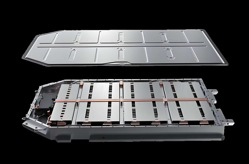
The battery pack enclosure was designed to house the electric vehicle battery modules, provide structural support, and protect the internal components from external forces and environmental factors. The enclosure consists of three main components manufactured from aluminum alloy (yield strength 370 MPa): an upper cover, a lower tray, and a surrounding frame structure. Two longitudinal beams divide the interior into three compartments corresponding to the battery modules, while side reinforcement ribs provide additional protection against lateral impacts. Four mounting lugs are positioned at the front and rear ends to secure the battery pack to the vehicle chassis.
For the finite element analysis, I employed the following modeling strategies to manage computational complexity while maintaining simulation accuracy:
- The thin-walled upper cover and lower tray were simplified using the mid-surface extraction technique, converting solid elements to shell elements to reduce element count.
- The battery modules were represented by concentrated mass points, as their detailed modeling would significantly increase computational cost without substantially affecting the structural analysis of the enclosure.
- The liquid cooling plate was included in the model because its structural integrity is critical—a failure could lead to coolant leakage and potential short circuits in the electric vehicle battery.
The final mesh contained 398,912 elements and 702,566 nodes, providing adequate resolution for accurate stress and deformation predictions.
Static Structural Analysis under Extreme Conditions
I evaluated the structural performance of the battery pack enclosure under three typical extreme loading conditions: sudden braking (3g longitudinal acceleration), sharp turning (3g lateral acceleration), and rough road driving (3g vertical acceleration). The mounting holes on the lugs served as fixed constraints. The simulation results are summarized in Table 20.
| Load Case | Maximum Deformation (mm) | Location of Max Deformation | Maximum Stress (MPa) | Location of Max Stress |
|---|---|---|---|---|
| Sudden braking | 0.09 | Liquid cooling plate corners | 17.18 | Mounting lugs |
| Sharp turning | 0.22 | Liquid cooling plate (side) | 17.62 | Mounting lugs |
| Rough road | 4.45 | Upper cover | 53.94 | Mounting lugs |
The results indicated that the enclosure exhibits excellent structural integrity under both the sudden braking and sharp turning conditions, with maximum stresses well below the material yield strength. However, under the rough road condition, the upper cover experienced a maximum deformation of 4.45 mm, which is relatively large and may cause interference with internal components or affect the sealing integrity of the enclosure.
Modal and Random Vibration Analysis
Modal analysis was performed to determine the natural frequencies of the battery pack enclosure. The first six modal frequencies are presented in Table 21.
| Mode | Natural Frequency (Hz) |
|---|---|
| 1 | 16.82 |
| 2 | 32.91 |
| 3 | 35.67 |
| 4 | 41.01 |
| 5 | 46.88 |
| 6 | 47.55 |
The first natural frequency was found to be 16.82 Hz, which is lower than the typical excitation frequency range of 30 Hz for road-induced vibrations in vehicles. This indicates a potential resonance risk, prompting the need for random vibration analysis to identify critical response regions.
The random vibration analysis followed the test conditions specified in GB 38031-2020 for electric vehicle battery packs. Table 22 summarizes the PSD input applied in the X, Y, and Z directions.
| Frequency (Hz) | X-direction PSD (g²/Hz) | Y-direction PSD (g²/Hz) | Z-direction PSD (g²/Hz) |
|---|---|---|---|
| 10 | – | 0.005 | – |
| 15 | – | – | 0.015 |
| 20 | – | 0.005 | – |
| 30 | – | – | 0.006 |
| 65 | – | – | 0.001 |
| 100 | – | – | 0.001 |
| 200 | 0.0001 | 0.00015 | 0.0003 |
The random vibration analysis results are summarized in Table 23. Under X-direction excitation, the maximum deformation was negligible. Under Y-direction excitation, the maximum deformation occurred in the liquid cooling plate (0.02 mm), with a maximum stress of 15.33 MPa in the longitudinal beams. Under Z-direction excitation, the upper cover experienced the maximum deformation of 13.65 mm, and the maximum stress was 62.46 MPa at the mounting lugs. While the stress values were all significantly below the yield strength, the upper cover deformation of 13.65 mm under Z-direction vibration was considered excessive and required design optimization.
| Direction | Maximum Deformation (mm) | Deformation Location | Maximum Stress (MPa) | Stress Location |
|---|---|---|---|---|
| X | Negligible | – | 0.04 | Upper cover |
| Y | 0.02 | Liquid cooling plate | 15.33 | Longitudinal beam |
| Z | 13.65 | Upper cover | 62.46 | Mounting lugs |
Shape Optimization of the Upper Cover
To improve the stiffness of the upper cover and reduce excessive deformation under vertical vibration, I employed the topography optimization method. This technique redistributes material in the design domain by moving grid nodes iteratively to enhance structural rigidity without adding material. The optimization setup defined the design domain as the central region of the upper cover, while the perimeter edges (which connect to the frame) were set as non-design regions to maintain the original mounting interfaces.
Figure 5.11(a) shows the topography optimization results amplified 20× for visualization. The optimization suggested four reinforcing ribs along the perimeter and two circular dimples in the diagonal positions of the upper cover. Based on these results, I created a simplified model suitable for practical manufacturing, incorporating the recommended stiffening features while maintaining manufacturability through the stamping process.
The optimized upper cover was simulated under the Z-direction random vibration condition. The results, shown in Figure 5.12, demonstrated a dramatic improvement: the maximum deformation was reduced from 13.65 mm to 0.01 mm, representing a reduction of 99.9%. This substantial enhancement in structural stiffness ensures that the upper cover will not interfere with internal battery components even under severe vibration conditions, thereby ensuring the safety and reliability of the electric vehicle battery pack.
Conclusions and Future Work
This article presented a comprehensive design and optimization study of a power battery pack for a new energy vehicle, focusing on the thermal management system and structural enclosure. The main conclusions can be summarized as follows:
First, the required battery capacity was determined as 40.5 kWh based on the target cruising range of 200 km and the NEDC driving cycle analysis. The maximum discharge rate of 3C was established to meet the vehicle’s power requirements, considering maximum speed, gradeability, and acceleration performance.
Second, the thermal analysis of the electric vehicle battery demonstrated that the battery temperature rises significantly with increasing discharge rates. At 3C discharge, the single cell temperature reached 53.41°C, which exceeds the safe operating range. This confirmed the necessity of implementing an active liquid cooling system.
Third, among the various liquid cold plate designs investigated, the parallel flow channel configuration with 5 channels and 25 mm channel width provided optimal cooling performance with the lowest flow resistance. The 50wt% ethylene glycol solution was selected as the most suitable coolant, balancing cooling efficiency with cold-weather operability.
Fourth, for 2C discharge conditions, a coolant flow rate of 0.06 kg/s was sufficient to maintain the battery temperature below 40°C. For 3C discharge conditions, a novel double-layer liquid cooling plate design was developed, successfully reducing the maximum battery temperature to 37.92°C with a temperature difference of only 2.6°C across the cells.
Fifth, parameter optimization using the NSGA-II algorithm reduced the flow resistance of the liquid cooling plate by 32.23%, from 962.88 Pa to 652.5 Pa, while maintaining excellent cooling performance. The optimized design minimized flow vortices in the merging regions and improved flow distribution uniformity.
Sixth, the structural analysis of the battery pack enclosure revealed adequate strength under static loads. However, the upper cover showed excessive deformation under rough road conditions (4.45 mm) and Z-direction random vibration (13.65 mm). Through topography optimization, the upper cover deformation was reduced to 0.01 mm, representing a 99.9% improvement in stiffness.
For future work, several aspects merit further investigation. First, the lumped battery model used in this study could be refined to account for the detailed internal structure, improving the accuracy of heat generation predictions. Second, experimental validation of the thermal management system should be conducted under controlled laboratory conditions to verify the simulation results. Third, the feasibility of lightweight materials such as carbon fiber composites for the battery pack enclosure should be explored from both performance and cost perspectives, potentially achieving additional weight reduction for the electric vehicle battery system.