
Electric vehicles heavily depend on traction batteries for energy storage and delivery. The cells must deliver high instantaneous power during acceleration and accept regenerative energy during braking, while remaining inside a safe and efficient temperature window. Lithium-ion chemistry offers high energy density and long cycle life, but it is also strongly temperature-dependent. When traction battery packs are discharged at high C-rates, heat is generated faster than it can be rejected from the compact module, causing a pronounced temperature rise. This rise accelerates side reactions, increases internal resistance, degrades capacity, shortens service life, and may ultimately initiate thermal runaway. Therefore, a robust thermal management system is not an accessory for traction batteries; it is a fundamental safety and performance requirement.
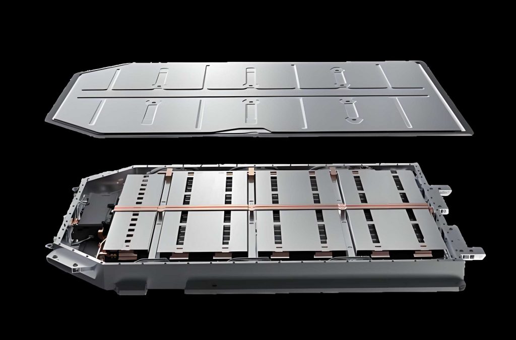
In my research, I focus on liquid cooling because it offers high heat-transfer coefficients, compact packaging, and controllable pumping-power requirements. Cold plates are widely used in traction battery thermal management systems because they provide large contact-area cooling and can be integrated between cells or beneath the module. However, conventional straight-channel cold plates often suffer from thick thermal boundary layers and limited mixing. An attractive improvement is to place pin fins inside the coolant channels. Pin fins break the continuous growth of the boundary layer, induce local flow separation and vortices, and therefore enhance heat transfer at the expense of a moderate pressure-drop penalty. The optimum pin-fin geometry must balance heat-transfer enhancement and pumping-power consumption, especially for large traction battery modules.
My study combines experimental characterization, CFD simulation, surrogate-model-based multi-objective optimization, and laboratory validation. I first established a validated heat-source model for a single lithium-ion cell. I then solved the conjugate heat-transfer problem for a traction battery module cooled by cold plates with straight channels and pin-fin arrays. After comparing square, circular, and triangular pin fins, I selected circular pin fins as the best compromise. I optimized the mass-flow rate, channel height, and pin-fin pitch with a Kriging surrogate and the NSGA-II algorithm. Finally, I fabricated a circular-pin-fin cold plate, constructed a single-phase flow and heat-transfer test rig, and measured pressure drop, temperature distribution, thermal resistance, and pumping-power consumption.
1. Single Traction Battery Cell Heat-Generation Model
Traction batteries are complex electrochemical systems. A typical lithium-ion cell contains positive and negative electrodes, current collectors, a porous separator, electrolyte, and a casing. During charging and discharging, lithium ions move from one electrode to the other while electrons circulate through an external circuit. In every charge-discharge cycle, several heat generation mechanisms appear: reversible entropy change, ohmic resistance, polarization, and side reactions. In normal operation, the irreversible heat caused by internal resistance dominates. I used the Bernardi heat-generation model to calculate volumetric heat-generation rate.
The general Bernardi expression is:
$$
q = \beta \frac{I}{V_c} \left[ (E_0 – U) – T \frac{dE_0}{dT} \right]
$$
where \( I \) is the applied current, \( V_c \) is the cell volume, \( E_0 \) is the open-circuit voltage, \( U \) is the terminal voltage, \( T \) is the cell temperature, and \( dE_0/dT \) is the temperature-entropy coefficient. In my simplified model, the reversible and polarization parts were assumed to be small relative to ohmic heating, and the volumetric heat-generation rate was reduced to:
$$
q = \frac{I^2 R_T}{V_c}
$$
where \( R_T \) is the total internal resistance. The value of \( R_T \) depends strongly on state of charge and temperature. I adopted a 100 Ah commercial prismatic lithium iron phosphate cell as the research object. Table 1 summarizes the physical parameters used in the model.
| Parameter | Value | Unit |
|---|---|---|
| Nominal capacity | 100 | Ah |
| Working voltage range | 2.5–3.65 | V |
| Cell dimensions | 160 × 116 × 50 | mm |
| Anisotropic thermal conductivity x/y/z | 1.5 / 22.5 / 22.5 | W m⁻¹ K⁻¹ |
| Cell mass | 1.65 | kg |
| Equivalent density | 2050 | kg m⁻³ |
| Specific heat capacity | 1088.75 | J kg⁻¹ K⁻¹ |
The transient heat conduction in the cell is governed by the energy equation:
$$
\rho_b c_b \frac{\partial T}{\partial t}
= k_{x,b} \frac{\partial^2 T}{\partial x^2}
+ k_{y,b} \frac{\partial^2 T}{\partial y^2}
+ k_{z,b} \frac{\partial^2 T}{\partial z^2}
+ q
$$
Because the cell is a layered composite, I determined its effective thermal properties using equivalent-resistance concepts. The through-plane thermal conductivity follows a series-resistance model, while the in-plane conductivities follow a parallel-resistance model:
$$
k_{T,x} = \frac{\sum L_i}{\sum \left( L_i / k_{T,i} \right)}
$$
$$
k_{T,y} = k_{T,z} = \frac{\sum L_i k_{T,i}}{\sum L_i}
$$
The density and specific heat of the homogenized cell are defined by:
$$
\rho_{cell} = \frac{\sum L_i \rho_i}{\sum L_i}
$$
$$
c_{cell} = \frac{\sum \left( \rho_i L_i \right) c_i}{\sum \rho_i L_i}
$$
I measured the internal resistance of the cell during a 1C discharge. Figure 2 in the original thesis shows that the resistance changes gently between 20% and 80% state of charge, but increases sharply outside that range. Therefore, I set the discharge depth to 80%, meaning that the simulation stopped at 20% state of charge. I fitted the resistance data with a polynomial function to create the user-defined heat-source function for CFD simulation.
I verified the single-cell thermal model by comparing the simulated temperature rise with experimental data. The simulation was performed in ANSYS Fluent using the Simplified Bernardi user-defined function. The predicted temperature at key checkpoints matched the measurements within 5%. This level of accuracy was acceptable for subsequent module-level simulations because the most important physical phenomena were captured: internal heat diffusion, heat accumulation, and surface convection to the environment.
2. Numerical Simulation of Pin-Fin Channel Cold Plates for Traction Battery Module
2.1 Geometry and Material Properties
After validation of the single-cell model, I developed a full-scale traction battery module cooled with three liquid cold plates. The module contains 24 prismatic cells. Each cell measures 160 mm by 116 mm by 50 mm. The cells are arranged in two rows, with twelve cells in each row. Silicone gap pads are placed between adjacent cells and between each cell and the cold plate to improve thermal contact and accommodate swelling. The cold plate has a length of 655 mm, a width of 134 mm, and a height of 14 mm. The internal cooling passages are 12 mm wide and 1.5 mm high. The plate is fed by one central inlet and two side outlets, creating eight parallel channels. This flow arrangement leads to uniform flow distribution across the width. Figure 1 in the previous text represented this concept schematically.
Inside the channels, I investigated three different pin-fin shapes: square, circular, and triangular pin fins. The pin fins were arranged in an in-line pattern. In every case, the pin diameter or equivalent hydraulic side length was 3 mm. The material properties used in the conjugate heat-transfer simulation are listed in Table 2.
| Component | Density (kg m⁻³) | Specific heat (J kg⁻¹ K⁻¹) | Thermal conductivity (W m⁻¹ K⁻¹) | Dynamic viscosity (Pa s) |
|---|---|---|---|---|
| Silicone gap pad | 2094.96 | 2684 | 4 | — |
| Aluminum cold plate | 2719 | 871 | 202.4 | — |
| 50% aqueous ethylene glycol | 1065 | 3281 | 0.38 | 0.0069 × (T / 273)⁻⁸·³ |
2.2 Governing Equations
I treated the coolant as incompressible and solved the steady-state conservation equations for the fluid domain. The continuity equation is:
$$
\frac{\partial \rho_f}{\partial t} + \nabla \cdot \left( \rho_f \mathbf{v} \right) = 0
$$
The momentum equation includes pressure and viscous forces:
$$
\frac{\partial}{\partial t} \left( \rho_f \mathbf{v} \right) + \nabla \cdot \left( \rho_f \mathbf{v} \mathbf{v} \right)
=
-\nabla P + \nabla \cdot \left[ \mu \left( \nabla \mathbf{v} + \left( \nabla \mathbf{v} \right)^T \right) \right]
$$
The energy equation for fluid convection and conduction is:
$$
\frac{\partial}{\partial t} \left( \rho_f c_f T_f \right) + \nabla \cdot \left( \rho_f c_f \mathbf{v} T_f \right)
=
\nabla \cdot \left( k_f \nabla T_f \right)
$$
For the solid regions, I used the heat-conduction equation:
$$
\frac{\partial}{\partial t} \left( \rho_s c_s T_s \right)
=
\nabla \cdot \left( k_s \nabla T_s \right)
$$
Straight channels kept laminar flow because the Reynolds number remained low. Pin-fin channels generated local recirculations and boundary-layer detachment, so I selected the standard \( k-\varepsilon \) turbulence model for those simulations. The transport equations for turbulence kinetic energy \( k \) and dissipation rate \( \varepsilon \) are:
$$
\frac{\partial \left( \rho k \right)}{\partial t}
+
\frac{\partial \left( \rho u_j k \right)}{\partial x_i}
=
\frac{\partial}{\partial x_j}
\left[
\left( \mu + \frac{\mu_t}{\sigma_k} \right)
\frac{\partial k}{\partial x_j}
\right]
+
P_k – \rho \varepsilon
$$
$$
\frac{\partial \left( \rho \varepsilon \right)}{\partial t}
+
\frac{\partial \left( \rho u_j \varepsilon \right)}{\partial x_i}
=
\frac{\partial}{\partial x_j}
\left[
\left( \mu + \frac{\mu_t}{\sigma_\varepsilon} \right)
\frac{\partial \varepsilon}{\partial x_j}
\right]
+
C_{\varepsilon 1} \frac{\varepsilon}{k} P_k
–
C_{\varepsilon 2} \rho \frac{\varepsilon^2}{k}
$$
The model constants are \( C_{\varepsilon 1}=1.44 \), \( C_{\varepsilon 2}=1.92 \), \( \sigma_k=1.0 \), and \( \sigma_\varepsilon=1.2 \).
2.3 Boundary Conditions and Mesh Independence
All cells in the module were energized by the same volumetric heat source at a 1C discharge rate. The discharge depth was 80% of the nominal capacity. The external surfaces of the battery module were subjected to natural convection with a heat-transfer coefficient of 10 W m⁻² K⁻¹. The inlet boundary was a mass-flow inlet with values between 0.01 kg/s and 0.03 kg/s. The outlet was a pressure-outlet at atmospheric pressure. The ambient and inlet coolant temperatures were 293 K. The no-slip condition was applied at the walls. I ignored the contact thermal resistances at the silicone pad interfaces, which is a common simplification in module-level thermal analysis.
I used the Poly-Hexcore mesh method in Fluent Meshing. This approach creates high-quality hexahedral cells in the core region and polyhedral cells near the walls. I carried out mesh-independence checks for the straight-channel and circular-pin-fin modules. For the straight-channel module, the maximum temperature and pressure drop stabilized after approximately 12.5 million cells. For the circular-pin-fin module, about 13.2 million cells were required. The final mesh sizes were therefore selected as 12.5 million and 13.2 million cells, respectively.
To validate the numerical model, I fabricated a smaller pin-fin cold plate and tested it in a closed-loop liquid-cooling bench. The verification plate had external dimensions of 213 mm by 148 mm by 14 mm, a channel height of 4 mm, pin-fin pitch of 15 mm, and pin-fin diameter of 3 mm. A heating film supplied a uniform heat flux of 36 W. I compared different turbulence models with the measured pressure drop. The standard \( k-\varepsilon \) model gave the smallest deviation from the measurements, with an average relative error of 7.1%. The predicted heating-surface average temperature was within 0.8 K of the measured value. Therefore, the standard \( k-\varepsilon \) model was selected for all pin-fin simulations.
2.4 Comparison of Straight and Pin-Fin Channel Cold Plates
I evaluated each cold-plate configuration using three metrics: maximum cell temperature \( T_{\mathrm{max}} \), maximum in-plane temperature difference \( \Delta T \), and pressure drop \( \Delta P \). These metrics directly relate to traction battery safety, temperature uniformity, and pumping power. Table 3 summarizes the geometry definitions and evaluation indicators.
| Symbol | Definition | Expression |
|---|---|---|
| \( T_{\mathrm{max}} \) | Maximum temperature in the cell domain | \( \max \{ T_1, T_2, \ldots, T_n \} \) |
| \( \Delta T \) | Temperature difference on the central mid-plane | \( T_{\mathrm{max,mid}} – T_{\mathrm{min,mid}} \) |
| \( \Delta P \) | Pressure drop across the cold plate | \( P_{\mathrm{in}} – P_{\mathrm{out}} \) |
At every mass-flow rate, all pin-fin cold plates removed heat more effectively than the straight channel. At 0.01 kg/s, the circular-pin-fin cold plate reduced the maximum temperature by 1.5 K compared with the straight channel. At 0.02 kg/s and 0.03 kg/s, the reductions increased to 2.5 K and 2.9 K, respectively. This trend confirms that turbulence promoters become increasingly valuable as the flow rate rises. Higher velocity increases the bulk convective ability, while pin fins maintain boundary-layer disruption along the entire channel length.
Table 4 compares the evaluated configurations according to heat-transfer capability, temperature uniformity, pressure drop, and overall balance.
| Configuration | Heat-transfer capability | Temperature uniformity | Pressure drop | Overall thermo-hydraulic balance |
|---|---|---|---|---|
| Straight channel (SC) | Lowest | Good only at very low flow | Lowest | Poor |
| Square pin fin (S-Pin-fin) | Highest | High at moderate/high flow | Highest | Moderate |
| Circular pin fin (C-Pin-fin) | High | High at moderate/high flow | Intermediate | Best |
| Triangular pin fin (T-Pin-fin) | Intermediate | High at moderate/high flow | Intermediate | Acceptable |
The square pin fin provided the lowest steady-state temperature because it had the smallest flow passage and caused the strongest turbulent mixing. However, it also caused the highest pressure drop. At 0.02 kg/s and 0.03 kg/s, the pressure drop of the square-pin-fin cold plate was 0.6 kPa and 1.2 kPa higher than that of the circular-pin-fin cold plate. The circular pin-fin channel achieved a maximum-temperature reduction of 2.9 K and a temperature-difference reduction of 0.7 K relative to the straight channel at 0.03 kg/s, while keeping the pressure drop lower than the square-pin-fin configuration. Therefore, I identified the circular pin-fin cold plate as the most promising design for traction battery thermal management.
2.5 Heat-Transfer Enhancement Mechanism
I investigated the velocity contours, heat-transfer coefficient contours, vortex structures, and turbulence-kinetic-energy fields to clarify why pin fins improve heat transfer. In the straight channel, high heat-transfer coefficients occurred only near the inlet. Once the boundary layer became fully developed, its thickness increased along the flow direction, and the local heat-transfer coefficient decayed significantly. Pin fins changed this behavior. As coolant flowed across a pin, the flow separated and created periodic vortices. Those vortices broke the boundary layer, increased local velocity fluctuations, and transported cooler fluid from the channel core toward the heated wall.
The circular pin-fin channel produced a regular chain of coherent, nearly circular vortices in the wake of each pin. The high heat-transfer regions were aligned with these vortices. The turbulence kinetic energy remained concentrated in the shear layers near the vortex cores, which allowed efficient use of turbulent kinetic energy without excessively large dissipation. The square pin-fin channel generated fragmented and unstable vortex structures. Although they produced high turbulence intensity and high heat-transfer coefficients, they also generated a large pressure drop because of severe vortex breakdown and dissipation. The triangular pin-fin channel showed a mixture of leading-edge shedding and trailing-edge reattachment. This behavior enhanced heat transfer, but less efficiently than the circular shape.
Hence, the circular pin fin offers the best compromise between convective enhancement and pressure-loss increase. This conclusion motivated the next step: multi-objective optimization of the circular-pin-fin cold plate for a complete traction battery module.
3. Multi-Objective Optimization of the Circular-Pin-Fin Cold Plate
3.1 Design Variables and Objective Functions
I selected three design variables for the circular-pin-fin cold plate: coolant mass-flow rate \( A \), channel height \( B \), and pin-fin pitch \( C \). These variables affect the heat-transfer coefficient, temperature uniformity, and pressure drop in different ways. Increasing the mass-flow rate enhances convective heat transfer but increases pumping power. Decreasing the channel height increases velocity and heat transfer for a fixed mass-flow rate but can dramatically increase pressure drop. Adjusting the pin-fin pitch changes the number of row interruptions and vortex-generation frequency. Table 5 lists the initial values and allowable ranges of the design variables.
| Design variable | Symbol | Initial value | Minimum | Maximum |
|---|---|---|---|---|
| Mass-flow rate (kg/s) | \( A \) | 0.0200 | 0.0100 | 0.0300 |
| Channel height (mm) | \( B \) | 1.5 | 1.5 | 4.0 |
| Pin-fin pitch (mm) | \( C \) | 15 | 4 | 30 |
Initially, I considered three objectives: maximum temperature \( T_{\mathrm{max}} \), temperature difference \( \Delta T \), and pressure drop \( \Delta P \). A correlation analysis showed that \( T_{\mathrm{max}} \) and \( \Delta T \) had a very strong positive correlation, with a Pearson coefficient of 0.99. Therefore, including both would add redundant information. I removed \( T_{\mathrm{max}} \) from the final optimization stage and used \( \Delta T \) and \( \Delta P \) as the two conflicting objectives. This reduced the dimensionality of the Pareto front and improved the efficiency of the optimizer.
3.2 Optimal Latin Hypercube Sampling and Kriging Surrogate Model
I used optimal Latin hypercube sampling to generate 31 points that uniformly cover the three-dimensional design space. Each design point was evaluated using the validated CFD model. Table 6 gives a representative subset of the sample matrix with the corresponding simulation results.
| No. | \( A \) (kg/s) | \( B \) (mm) | \( C \) (mm) | \( T_{\mathrm{max}} \) (K) | \( \Delta T \) (K) | \( \Delta P \) (kPa) |
|---|---|---|---|---|---|---|
| 1 | 0.0260 | 2.16 | 23.6 | 307.2 | 4.4 | 2.2 |
| 2 | 0.0167 | 2.34 | 17.3 | 309.5 | 6.2 | 1.0 |
| 3 | 0.0127 | 1.92 | 22.2 | 311.3 | 7.6 | 0.9 |
| 4 | 0.0293 | 1.76 | 13.8 | 306.7 | 4.1 | 4.2 |
| 5 | 0.0153 | 1.50 | 15.2 | 309.8 | 6.6 | 2.1 |
| 6 | 0.0273 | 2.92 | 11.7 | 307.0 | 4.3 | 1.9 |
| 7 | 0.0140 | 2.66 | 5.4 | 310.5 | 7.0 | 0.8 |
| 8 | 0.0207 | 1.66 | 20.8 | 308.2 | 5.2 | 2.4 |
| … | … | … | … | … | … | … |
| 31 | 0.0100 | 3.34 | 8.9 | 313.3 | 8.7 | 0.3 |
I constructed a Kriging surrogate model to map the design variables to \( \Delta T \) and \( \Delta P \). The Kriging model provides both a predicted mean and an estimate of prediction uncertainty. I evaluated the accuracy using the coefficient of determination:
$$
R^2 = 1 – \frac{\sum_{i=1}^{n} \left( y_i – \hat{y}_i \right)^2}{\sum_{i=1}^{n} \left( y_i – \bar{y} \right)^2}
$$
The cross-validation results gave \( R^2 = 0.966 \) for \( \Delta T \) and \( R^2 = 0.952 \) for \( \Delta P \). Both values were above 0.95, which indicates that the surrogate model was sufficiently accurate for optimization.
3.3 Sensitivity and Correlation Analysis
I calculated the sensitivity index of each objective with respect to each design variable:
$$
S_{A_i} = \frac{f_{\mathrm{max}}(x_i) – f_{\mathrm{min}}(x_i)}{f_{\mathrm{max}}(x) – f_{\mathrm{min}}(x)} \times 100\%
$$
The results show that mass-flow rate has a dominant influence on both \( T_{\mathrm{max}} \) and \( \Delta T \), with sensitivity values of 99.6% and 98.8%, respectively. Channel height is the dominant factor for pressure drop, with a sensitivity of 44.2%. Pin-fin pitch has a weak effect on pressure drop, with a sensitivity of only 2.8%. These findings are important because they indicate that flow-rate adjustments are the most direct way to control the thermal state of a traction battery module, while channel-height changes are the most effective way to manage pumping-power consumption. Table 7 summarizes the sensitivity values.
| Objective | Mass-flow sensitivity | Channel-height sensitivity | Pin-pitch sensitivity |
|---|---|---|---|
| \( T_{\mathrm{max}} \) | 99.6% | Low | Low |
| \( \Delta T \) | 98.8% | Low | Low |
| \( \Delta P \) | — | 44.2% | 2.8% |
Correlation analysis between objectives showed a clear trade-off between the thermal objective and hydraulic objective. The correlation coefficients were \( -0.70 \) between \( \Delta P \) and \( T_{\mathrm{max}} \), and \( -0.67 \) between \( \Delta P \) and \( \Delta T \). This means that a design that reduces the maximum temperature also tends to increase the pressure drop. Because \( T_{\mathrm{max}} \) and \( \Delta T \) were strongly positively correlated, I used only \( \Delta T \) and \( \Delta P \) in the final optimization formulation. This simplified the problem and reduced the computational effort without losing meaningful design information.
3.4 NSGA-II Optimization
I used the non-dominated sorting genetic algorithm NSGA-II to search for the Pareto-optimal front. NSGA-II is particularly suitable for two-objective thermal-fluid problems because it preserves diversity and guarantees the retention of elite solutions. I set the population size to 120 and ran the algorithm for 50 generations. The optimizer evaluated 6000 candidate designs using the Kriging surrogate model. The result was a Pareto front with a clear trade-off between temperature uniformity and pressure drop.
I selected three representative designs from the Pareto front and simulated them with the full CFD model. Table 8 compares the surrogate predictions and CFD results with the baseline cold plate design.
| Case | \( A \) (kg/s) | \( B \) (mm) | \( C \) (mm) | \( T_{\mathrm{max}} \) (K) | \( \Delta T \) (K) | Prediction error | \( \Delta P \) (kPa) | Prediction error | Improvement in \( \Delta T \) | Improvement in \( \Delta P \) |
|---|---|---|---|---|---|---|---|---|---|---|
| Baseline | 0.0200 | 1.5 | 15 | 308.3 | 5.40 | — | 3.10 | — | — | — |
| CFD-1 | 0.0253 | 3.66 | 22 | 307.5 | 4.51 | 0.9% | 1.27 | 1.6% | 16.5% | 59.0% |
| CFD-2 | 0.0285 | 3.14 | 19 | 306.9 | 4.15 | 3.1% | 1.76 | 0.6% | 23.1% | 43.2% |
| CFD-3 | 0.0294 | 2.52 | 18 | 306.7 | 4.07 | 3.4% | 2.30 | 1.7% | 24.6% | 25.8% |
The CFD results matched the surrogate predictions within 3.4% for temperature difference and within 1.7% for pressure drop. This agreement verified the reliability of the Kriging-based optimization framework. The first design, CFD-1, was the best from the viewpoint of energy consumption because it reduced pressure drop by 59.0% while still improving temperature uniformity by 16.5%. The third design, CFD-3, was the best from the viewpoint of thermal performance because it reduced temperature difference by 24.6% while still reducing pressure drop by 25.8%. The second design, CFD-2, offered the most balanced compromise: it reduced the temperature difference by 23.1%, from 5.40 K to 4.15 K, and reduced the pressure drop by 43.2%, from 3.10 kPa to 1.76 kPa. I therefore selected CFD-2 as the final optimized design for the circular-pin-fin cold plate.
3.5 Performance Evaluation of the Optimized Cold Plate
Thermal resistance provides a direct physical interpretation of the heat-removal path. I decomposed the total thermal resistance into convective, heat-absorption, and conductive components:
$$
R_{\mathrm{conv}} = \frac{T_{\mathrm{ave}} – T_{\mathrm{liq}}}{q}
$$
$$
R_{\mathrm{heat}} = \frac{T_{\mathrm{out}} – T_{\mathrm{in}}}{q}
$$
$$
R_{\mathrm{cond}} = \frac{L_b}{k_s A_{\mathrm{cont}}}
$$
$$
R_{\mathrm{total}} = R_{\mathrm{conv}} + R_{\mathrm{heat}} + R_{\mathrm{cond}}
$$
where \( T_{\mathrm{ave}} \) is the average cell surface temperature, \( T_{\mathrm{liq}} \) is the average coolant temperature, \( q \) is the steady-state heat-generation rate, \( T_{\mathrm{in}} \) and \( T_{\mathrm{out}} \) are the inlet and outlet coolant temperatures, \( L_b \) is the cold-plate thickness, \( k_s \) is the solid thermal conductivity, and \( A_{\mathrm{cont}} \) is the wetted area.
The convective resistance dominated the total thermal resistance. Compared with the straight-channel cold plate, the optimized circular-pin-fin cold plate reduced the total thermal resistance by 14% at 0.02 kg/s and by 16% at 0.03 kg/s. The decrease was attributed mainly to the lower convective thermal resistance caused by pin-fin-induced vortex mixing. The optimized cold plate had a slightly higher thermal resistance than the baseline circular-pin-fin plate because the optimized plate used taller channels and larger pin pitches, which reduced the flow velocity. However, the increase was negligible compared with the large saving in pressure drop.
I also evaluated the effective heat-transfer enhancement factor, which compares the heat-transfer improvement with the pressure-drop penalty under equal pumping-power conditions:
$$
p_f = \frac{Nu / Nu_0}{\left( \Delta P / \Delta P_0 \right)^{1/3}}
$$
Here, \( Nu \) is the Nusselt number and \( Nu_0 \) and \( \Delta P_0 \) are the reference Nusselt number and pressure drop of the baseline model. The Nusselt number is defined as:
$$
Nu = \frac{h_{\mathrm{ave}} D_h}{k_{\mathrm{liq}}}
$$
where \( D_h \) is the hydraulic diameter and \( k_{\mathrm{liq}} \) is the coolant thermal conductivity. At 0.02 kg/s, the optimized cold plate increased the Nusselt number by more than six times relative to the straight channel, and increased \( p_f \) by more than seven times. Compared with the baseline circular-pin-fin cold plate, the optimized cold plate improved \( Nu \) by 33.9% and \( p_f \) by 97.5%. When the flow rate increased from 0.02 kg/s to 0.03 kg/s, all configurations showed higher Nusselt numbers, but the enhancement factor decreased because the pressure-drop penalty grew faster than the heat-transfer improvement.
Finally, I defined a cooling-efficiency factor that compares the heat removed by the coolant to the hydraulic pumping power required to move the coolant:
$$
Q_{\mathrm{liq}}(t) = c_\mathrm{p} m \Delta T
$$
$$
Q_{\mathrm{cell}}(t) = \int_{t_0}^{t_1} I^2 R(t) \mathrm{d}t
$$
$$
\eta = \frac{Q_{\mathrm{liq}}(t) / t}{\Delta P \; q_v}
$$
where \( \Delta T \) is the coolant temperature rise, \( q_v \) is the volumetric-flow rate, \( m \) is the mass-flow rate, and \( t \) is the simulated time interval. The optimized cold plate reached \( \eta = 15452 \) at a mass-flow rate of 0.02 kg/s. This value was much higher than the straight-channel cold plate and roughly three times higher than the baseline circular-pin-fin design. At 0.03 kg/s, the baseline circular-pin-fin design showed the lowest cooling-efficiency factor, approximately 1823, because both the volumetric-flow rate and the pressure drop increased substantially. The optimized cold plate remained the most efficient configuration at both flow rates.
4. Experimental Study of the Circular-Pin-Fin Cold Plate
4.1 Effect of Channel Height
The optimized multi-objective result indicated a channel height of 3.14 mm. However, for real traction battery packaging, a thinner cold plate is desirable because it reduces the overall module volume and weight. Therefore, I performed an additional numerical study to examine whether a smaller channel height could preserve the thermal performance while reducing the plate thickness.
In those simulations, the mass-flow rate was kept at 0.0285 kg/s, the pin-fin pitch was 19 mm, and the pin-fin diameter was 3 mm. The channel height was varied from 1 mm to 4 mm. The maximum cell temperature increased by only 0.3 K over this entire range. The temperature difference was almost unchanged and reached its minimum at 1.5 mm. In contrast, the pressure drop decreased sharply as the channel height increased. Increasing the channel height from 1 mm to 1.5 mm reduced the pressure drop by 7.7 kPa, or 59.2%. Further increases in channel height produced diminishing returns. I concluded that a channel height of 1.5 mm provides excellent thermal performance, a very low pressure drop, and a compact structure for integration into traction battery packs. I selected this height for the experimental cold plate and named it the C-Pin-fin (BCS) model.
Because the geometry of this cold plate differs from the small validation plate used earlier, I re-validated the numerical model against laboratory data. In this validation, four heating films produced a total heating power of 280 W, the inlet temperature was 20 °C, and the mass-flow rate ranged from 0.005 kg/s to 0.03 kg/s. The pressure-drop prediction had a maximum relative error of 8%, and the average heating-surface temperature had a maximum error of 1.2 K. Thus, the numerical model accurately represented the C-Pin-fin (BCS) cold plate.
4.2 Cold Plate Fabrication and Experimental Platform
I manufactured the C-Pin-fin (BCS) cold plate by computer numerical control machining. Subtractive machining was selected because of its mature process, low cost for a large plate, high dimensional accuracy, and good surface finish. The manufactured cold plate had external dimensions of 732 mm by 191 mm by 12 mm. The inlet and outlet diameters were 6 mm. The internal channel height was 1.5 mm. The pin-fin pitch was 19 mm and the pin diameter was 3 mm. Four heating films, each with dimensions of 150 mm by 116 mm, were attached to the outer surface of the cold plate to provide a controlled heat load.
I built a closed-loop experimental bench to measure the single-phase flow and heat-transfer characteristics of this cold plate. The primary instruments included a gear pump, a liquid turbine flow meter, PT100 temperature sensors, pressure transmitters, K-type thermocouples, an infrared thermal camera, a constant-temperature water bath, a programmable DC power supply, and a data-acquisition system. The coolant was 50% aqueous ethylene glycol, which is commonly used in automotive traction battery cooling systems. Table 9 lists the measurement accuracy and range of each instrument.
| Instrument | Accuracy / Range |
|---|---|
| DC power supply | 0–200 W |
| Infrared thermal camera | ±2%, –20 to 2000 °C |
| Liquid turbine flow meter | ±0.5%, 0–10 L/min |
| Constant-temperature water bath | ±0.75%, –20 to 100 °C |
| Temperature sensor | ±1%, –100 to 280 °C |
| Inlet pressure transmitter | ±0.5%, 0–500 kPa |
| Outlet pressure transmitter | ±0.5%, 0–130 kPa |
The total heating power supplied by the films was calculated from the measured voltage and current:
$$
P_h = 8 U I_h
$$
where the factor eight accounts for the series-parallel connection of the four heating films used in the experiments. The effective heat flux applied to the cold plate was:
$$
q = \frac{c_p m \Delta T}{A}
$$
where \( A \) is the total wetted or film area. The pumping power required by the test section was:
$$
P_p = \Delta P q_v
$$
4.3 Uncertainty Analysis
Experimental results inevitably include instrument errors and random variations. I used standard error-propagation formulas to estimate the maximum relative uncertainty of derived quantities:
$$
\delta R = \sqrt{ \sum_{i=1}^{n} \left( \frac{\partial R}{\partial v_i} \delta v_i \right)^2 }
$$
$$
\xi_R = \frac{\delta R}{R}
$$
The individual measurement uncertainties were used in these equations. For example, the temperature sensor uncertainty was 0.5 °C; with a minimum measured temperature of 20 °C, the relative uncertainty was 2.5%. The inlet pressure transmitter had an uncertainty of 2.4% at the measured inlet pressure, while the outlet transmitter had 0.6% uncertainty. These values led to an uncertainty of 2.5% for pressure drop. Table 10 summarizes the maximum relative uncertainties for the main experimental parameters.
| Parameter | Maximum relative uncertainty |
|---|---|
| Inlet pressure \( P_{\mathrm{in}} \) | 2.4% |
| Outlet pressure \( P_{\mathrm{out}} \) | 0.6% |
| Volumetric-flow rate \( q_v \) | 2.5% |
| Mass-flow rate \( m \) | 2.5% |
| Coolant temperatures \( T_{\mathrm{in}}, T_{\mathrm{out}} \) | 1.6% |
| Pressure drop \( \Delta P \) | 2.5% |
| Heat flux \( q \) | 3.1% |
| Thermal resistance \( R \) | 3.6% |
4.4 Flow Resistance Results
I first measured the pressure drop of the C-Pin-fin (BCS) cold plate as a function of coolant volume-flow rate. No electrical power was supplied to the heating films during the pressure-drop tests. The inlet temperature was held at 293 K by the constant-temperature bath.
The experimental results show that pressure drop increases continuously with flow rate. The rate of increase is not constant. In the low-flow region, the pressure drop increases slowly because viscous effects dominate and the flow remains attached around the pin fins. As the flow rate increases, inertial forces become stronger, boundary-layer separation develops behind each pin, and wake recirculation grows. This leads to a faster increase in pressure drop. In the high-flow region, the pressure drop rises steeply because vortex shedding and turbulent mixing become fully developed. Even at the highest tested flow rate, the pressure drop of the C-Pin-fin (BCS) cold plate remained within the acceptable range for a practical traction battery cooling circuit.
4.5 Heat-Transfer Performance Results
I performed heat-transfer experiments at heating-film powers of 200 W, 280 W, 360 W, and 440 W. For each heating power, I varied the coolant mass-flow rate across the same range as the hydraulic tests. I obtained infrared thermal images of the heating-film surface during steady-state operation.
Figure 5 in the original thesis shows a typical infrared image. The heating-film temperature increased gradually along the direction of coolant flow. Near the inlet, the coolant temperature is low, the thermal boundary layer is thin, and the convective heat-transfer coefficient is high. The wall temperature is therefore relatively low. As the coolant moves downstream, it absorbs heat and its temperature rises. The local temperature difference between the wall and the coolant decreases, so the heating-film temperature increases. This is a well-known inlet-effect phenomenon.
At a constant flow rate, the heating-film temperature increased when the heat flux increased. At a constant heat flux, increasing the flow rate reduced the heating-film temperature because higher velocity enhanced the convective heat-transfer coefficient and carried away more heat. Two of the heating films, one near the inlet and one near the outlet, clearly illustrated this effect. The film located closer to the inlet was always cooler than the downstream film. The difference was caused by the higher local heat-transfer coefficient in the thermal entrance region. These observations confirm that the circular-pin-fin cold plate provides strong convective cooling but that the entrance effect remains important in long traction battery modules.
I also calculated the thermal resistance and pumping-power consumption for all tested operating points. As the coolant flow rate increased, the pumping power increased almost exponentially because both the flow rate and the pressure drop increased. At the same time, the thermal resistance decreased because higher velocity reduced the thermal boundary-layer thickness and enhanced mixing. The reduction in thermal resistance was large at the beginning and became smaller at high flow rates.
When the heating-film power increased, the thermal resistance often decreased slightly before stabilizing. This behavior is caused by the temperature dependence of the coolant physical properties. Higher surface temperatures reduce the viscosity of the aqueous ethylene glycol mixture, increase its thermal conductivity, and improve the convective heat-transfer coefficient. As the heating power increases further, the property changes saturate and the thermal resistance reaches a nearly constant value.
These results highlight an important design principle for traction battery thermal management: increasing coolant flow too much produces diminishing thermal benefits while consuming significantly more pumping power. A rational design should operate near the knee point of the thermal-resistance-versus-flow curve.
5. Summary and Conclusions
In this dissertation, I have systematically investigated the single-phase flow and heat-transfer characteristics of pin-fin channel cold plates for traction battery thermal management. The main conclusions are summarized below.
First, a validated single-cell heat-generation model was established using the Bernardi approach and measured internal-resistance data. The maximum prediction error of the single-cell temperature-rise simulation was within 5%. This model provided a reliable foundation for module-level conjugate heat-transfer simulations.
Second, I compared straight, square-pin, circular-pin, and triangular-pin cold-plate channels. All pin-fin configurations outperformed the straight channel. The circular pin-fin cold plate showed the best overall thermo-hydraulic balance. At a mass-flow rate of 0.03 kg/s, the circular-pin-fin cold plate reduced the maximum cell temperature by 2.9 K and the temperature difference by 0.7 K relative to the straight-channel cold plate. The heat-transfer enhancement mechanism was attributed to periodic flow separation, boundary-layer disruption, vortex generation, and efficient use of turbulent kinetic energy. The circular pin produced coherent vortices, while the square pin produced excessive turbulence and dissipation, leading to higher pressure drop.
Third, a Kriging-based multi-objective optimization was performed with NSGA-II. The optimal Latin hypercube design generated 31 sample points. The Kriging surrogate achieved high accuracy with \( R^2 = 0.966 \) for temperature difference and \( R^2 = 0.952 \) for pressure drop. Sensitivity analysis showed that mass-flow rate is the dominant factor controlling cell temperature, while channel height is the dominant factor controlling pressure drop. The selected optimum design used a mass-flow rate of 0.0285 kg/s, a channel height of 3.14 mm, and a pin-fin pitch of 19 mm. Relative to the baseline design, the optimized cold plate reduced temperature difference by 23.1% and pressure drop by 43.2%. The optimized cold plate also demonstrated lower thermal resistance than the straight channel, an effective heat-transfer enhancement factor much greater than one, and a maximum cooling-efficiency factor of 15452 at 0.02 kg/s.
Fourth, channel-height analysis showed that 1.5 mm is an excellent compact choice. Increasing the channel height from 1 mm to 1.5 mm reduced pressure drop by 59.2% while the maximum cell temperature increased by only 0.3 K. I fabricated a large circular-pin-fin cold plate with 1.5 mm channel height using subtractive manufacturing and tested it experimentally. The measured pressure-drop trend matched the numerical prediction with a maximum relative error of 8%, and the average heating-surface temperature matched within 1.2 K. Experimental results confirmed that pressure drop increases with flow rate and that flow resistance increases more rapidly at high flow rates. Heating-film temperature increases with heat flux and decreases with coolant flow rate. The spatial temperature distribution is strongly affected by the entrance effect. Finally, thermal resistance decreases with increasing flow rate and heating power, while pump-power consumption rises rapidly. A balanced choice of operating parameters is essential for achieving efficient and safe traction battery cooling.
Overall, this work demonstrates that a circular-pin-fin channel cold plate can provide excellent cooling performance and acceptable pumping power for traction batteries. The combination of validated simulation, surrogate-assisted multi-objective optimization, and experimental verification offers a practical framework for developing high-performance liquid cooling systems. Future work should include extreme temperature conditions, higher discharge rates, and the use of real battery modules with cycling protocols to further validate and refine the design.