
I present a comprehensive study on the temperature–energy synergistic thermal management of traction batteries in pure electric vehicles. My goal is to resolve the intrinsic conflict between precise battery temperature control and energy consumption of auxiliary thermal components. I first establish a coupled electro-thermal model of a lithium-ion traction battery and construct a layered thermal management architecture with coolant, radiator, and refrigeration circuits. The model is calibrated and validated using experiments on open-circuit voltage, hybrid pulse power characterization, thermal property tests, and heat exchanger bench tests. A key-factor screening is then conducted using optimal Latin hypercube sampling combined with variance analysis. Finally, I develop environment-specific control algorithms, including PID for low-temperature heating, nonlinear model predictive control for normal-temperature cooling, and grey-wolf-optimizer-based nonlinear model predictive control for high-temperature cooling. Simulation results in New European Driving Cycle demonstrate that the proposed strategies maintain the traction battery around the target temperature while reducing system energy consumption significantly compared with conventional threshold and PID control. The results highlight the necessity of coordinated management of compressors, pumps, fans, and heaters for the safe and efficient operation of electric vehicles.
Keywords: traction battery; thermal management; temperature–energy synergy; optimal Latin hypercube sampling; nonlinear model predictive control; grey wolf optimization.
1. Introduction
Environmental concerns and the exhaustion of fossil fuels have accelerated the transition toward electric mobility. Among the various technologies, pure electric vehicles equipped with lithium-ion traction batteries have become a promising solution for reducing greenhouse gas emissions and improving energy efficiency. During the last decade, the sales of electric vehicles in China have grown dramatically, and traction battery technology has been developed rapidly. Nevertheless, the application of traction batteries still faces two crucial challenges: thermal safety and range degradation under aggressive thermal loads.
A lithium-ion traction battery generates heat during charge and discharge. If the heat is not removed promptly, the battery temperature may exceed the permitted range. The optimum operating window of most traction batteries is between 25 ℃ and 40 ℃, while the temperature difference across the pack should be kept within 5 ℃. When the local temperature exceeds a critical value, internal exothermic side reactions accelerate, posing the risk of thermal runaway and catastrophic fire. Conversely, low temperature increases the internal resistance and reduces the usable energy and power of the traction battery. The heat management system therefore plays a central role in guaranteeing safety, performance, and lifetime.
Research on traction battery thermal management has mainly followed four paths: air cooling, liquid cooling, phase-change material cooling, and direct refrigerant cooling. Air-cooled systems are simple but have limited heat-transfer capability. Phase-change materials offer passive temperature buffering but suffer from low thermal conductivity. Direct refrigerant cooling is efficient but introduces complex plumbing and control. Indirect liquid cooling using cold plates has become the dominant configuration in production vehicles because it combines compact structure, acceptable cost, and high cooling efficiency. In my work, I focus on an indirect liquid-cooled traction battery thermal management system that is integrated with a cabin refrigeration circuit through a chiller.
Numerous control strategies have been investigated for traction battery thermal management. Threshold control is simple and robust, but it often causes temperature overshoot and frequent on–off switching. PID control is widely applied in industry due to its ease of implementation, yet it lacks the ability to handle strongly coupled nonlinear systems with multiple inputs and outputs. Fuzzy logic controllers can encode expert rules but require laborious calibration. Model predictive control has become attractive for traction battery thermal management because it can anticipate future thermal behavior, incorporate constraints, and optimize energy consumption over a receding horizon. However, the strong nonlinearities and conflicting objectives of the battery-thermal system demand a nonlinear predictive framework and efficient numerical solvers. Many previous studies concentrated on temperature regulation alone, while the energy penalty of the thermal management system was treated as a secondary issue. Therefore, my study aims to establish a temperature-and-energy coordinated strategy for traction batteries by combining a validated simulation platform, a statistical factor-screen method, and advanced nonlinear controllers.
2. Theoretical Modeling and Architecture of the Traction Battery Thermal Management System
2.1 Traction battery structure and operating principle
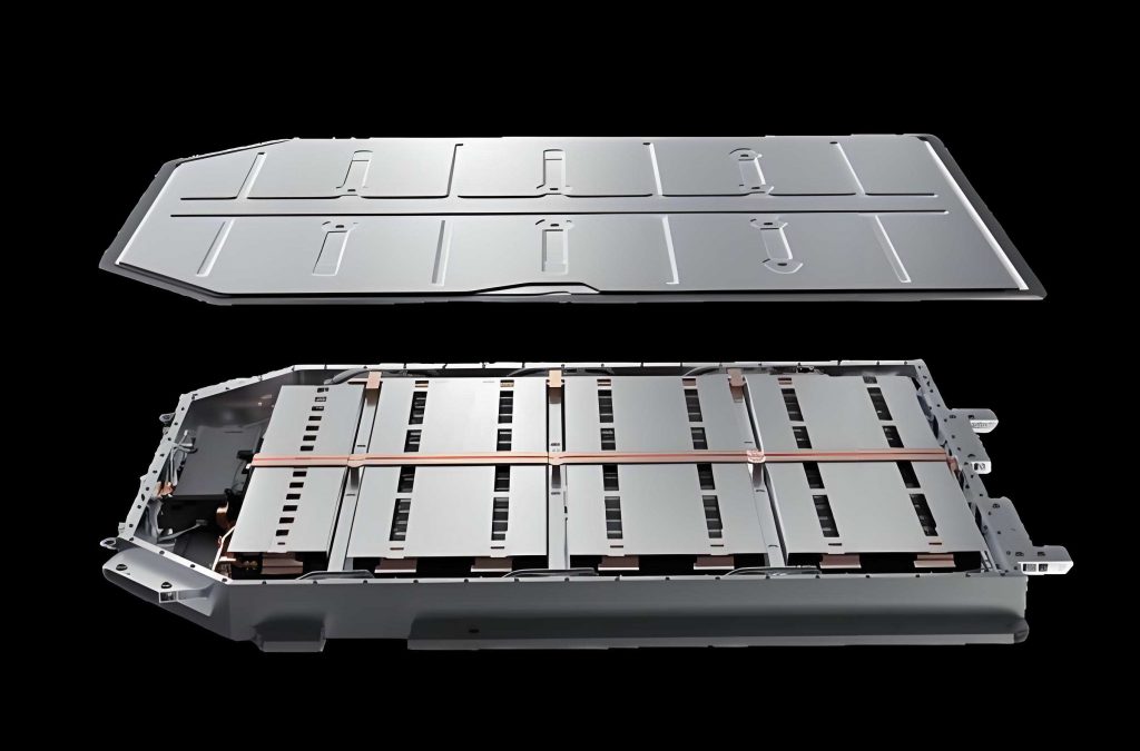
The traction battery considered in this study is a lithium iron phosphate cell. A lithium-ion cell consists of a positive electrode, a negative electrode, an electrolyte, a separator, and a metallic or laminated casing. During discharge, lithium ions de-intercalate from the negative graphite electrode, migrate through the electrolyte, and intercalate into the positive electrode. During charging, the migration is reversed. The redox reactions are:
$$ \mathrm{LiFePO_4} – x\mathrm{Li^+} – x e^- \rightleftharpoons x\mathrm{FePO_4} + (1-x)\mathrm{LiFePO_4} $$
$$ 6\mathrm{C} + x\mathrm{Li^+} + x e^- \rightleftharpoons \mathrm{Li_x C_6} $$
The reversible intercalation/deintercalation process gives rise to heat generation. To design a thermal management system for the traction battery pack, the heat source intensity and heat-transfer paths must be quantified.
2.2 Heat generation and heat-transfer models for the traction battery
The total heat generation inside a traction battery can be divided into reaction heat \(Q_r\), polarization heat \(Q_p\), Joule heat \(Q_j\), and side-reaction heat \(Q_s\). Since side-reaction heat is often negligible under normal conditions, I simplify the total heat as:
$$ Q = Q_r + Q_p + Q_j $$
The reaction heat is related to the entropic change during intercalation and can be written as \(Q_r = n m Q_e I / (M F)\), where \(n\) is the number of cells, \(m\) is the electrode mass, \(Q_e\) is the reaction heat, \(I\) is the current, \(M\) is the molar mass, and \(F\) is Faraday’s constant. The Joule and polarization heat are generally represented by the equivalent internal resistance \(R_e\). I use the Bernardi energy-balance equation to compute the heat-generation rate of the traction battery:
$$ \dot{q}_{\mathrm{gen}} = I\left( I R_e – T_b \frac{dU_{\mathrm{op}}}{dT_b} \right) $$
where \(T_b\) is the battery temperature, \(U_{\mathrm{op}}\) is the open-circuit voltage, and \(dU_{\mathrm{op}}/dT_b\) is the entropic coefficient. This model captures both irreversible resistive heating and reversible entropic heating.
Heat transfer from the traction battery to its surroundings occurs through conduction, convection, and radiation. Conduction inside the battery pack follows Fourier’s law:
$$ Q_f = -\lambda \frac{\partial T}{\partial x} $$
Convection at the interface between the battery and the cooling plate or surrounding air is expressed by Newton’s law of cooling:
$$ Q_a = h\left(T_b – T_c\right) $$
where \(T_c\) is the coolant temperature and \(h\) is the convection coefficient. Radiation is governed by the Stephan–Boltzmann equation:
$$ \phi = \varepsilon A \sigma T^4 $$
In the liquid-cooling plate, the equivalent heat-transfer coefficient is correlated with the flow regime. I adopt the following empirical relations:
$$ h = \frac{Nu\lambda}{d}, \quad Nu = 0.023 Re^{0.8}Pr^{0.3}, \quad Re = \frac{u d}{\mu} $$
where \(Nu\), \(Re\), and \(Pr\) are the Nusselt, Reynolds, and Prandtl numbers, respectively; \(u\) is the coolant velocity; \(d\) is the hydraulic diameter; \(\mu\) is the kinematic viscosity; and \(\lambda\) is the coolant conductivity. Because the detailed internal temperature distribution is not required in the control-oriented model, I use a lumped-parameter approach for the traction battery pack.
2.3 Heat-load estimation
To size the thermal components, I estimate the peak heat loads of the traction battery. Under a severe driving scenario in which the vehicle continues to run at 120 km/h for 1000 s, the total battery heat-generation rate can be computed approximately from the traction power:
$$ Q_{\mathrm{gen}} = n_p n_s q_{\mathrm{gen}}, \quad q_{\mathrm{gen}} = \left(\frac{P_{\mathrm{driv}}}{n_p \eta_b U}\right)^2 R $$
where \(n_p\) = 8, \(n_s\) = 125, \(U\) = 400 V, \(\eta_b\) = 0.86, and \(R\) = 0.03 Ω. The resultant heat-generation power is approximately 2474 W. The total cooling demand, which combines sensible heat and heat generation, is:
$$ Q_n = \frac{c_{p,b}(T_u – T_d) + Q_{\mathrm{gen}}}{t} $$
Using \(c_{p,b}\) = 1250 J/(kg·℃), \(T_u\) = 40 ℃, \(T_d\) = 30 ℃, and \(t\) = 1000 s, I obtain \(Q_n \approx 3457\) W. For cold-climate operation, the heating power needed to raise the battery temperature from −10 ℃ to 20 ℃ within 1500 s is calculated as:
$$ Q_h = \frac{c_{p,b}(T_d – T_u)}{t} $$
which gives approximately 1886 W. These values provide quantitative boundaries for the selection of the compressor, heater, pumps, and fans.
2.4 Vehicle powertrain modeling and thermal management architecture
To simulate realistic load conditions of a traction battery, I construct a pure electric vehicle model using a one-dimensional simulation environment. The vehicle is a front-driven or rear-driven configuration with a driver model that follows a prescribed speed trajectory, a motor model, and a longitudinal vehicle dynamics model. The main parameters of the vehicle model are listed below.
| Parameter | Symbol | Value | Unit |
|---|---|---|---|
| Vehicle mass | \(m_{veh}\) | 1445 | kg |
| Rolling resistance coefficient | \(f\) | 0.01 | – |
| Drag coefficient | \(C_D\) | 0.31 | – |
| Frontal area | \(A_c\) | 2.09 | m² |
| Rotational inertia factor | \(\delta\) | 1.4 | – |
The traction battery thermal management system designed in this study has a layered indirect architecture. The system consists of a coolant loop, a battery radiator loop, and a refrigeration loop. A two-position three-way valve connects the radiator branch to the coolant loop. A positive temperature coefficient heater is placed in the coolant loop for cold-start heating. The refrigeration loop consists of a compressor, a condenser, an expansion valve, and a chiller, where the refrigerant exchanges heat with the coolant that passes through the battery cold plate. The battery heat can be dissipated through the radiator with an electric fan or through the chiller with the chiller circuit depending on operating mode and ambient temperature.
For different ambient temperature ranges I define three operating modes. In cold environments, the PTC heater raises the coolant temperature and the circulation pump transfers heat to the traction battery. In mild or normal environments, the battery is cooled only by the radiator and fan when necessary, whereas the compressor is not operated. In hot environments, the chiller must be used to achieve stronger cooling and maintain the traction battery near the desired temperature. The boundary temperatures for modes are 5 ℃ and 30 ℃ in this study.
3. Physical Modeling and Model Validation of the Traction Battery Thermal Management System
3.1 Electro-thermal coupled model of the traction battery
For the traction battery simulation model, I use the Rint equivalent circuit model, which contains an ideal voltage source \(U_{\mathrm{op}}\) and a series resistance \(R_e\). The terminal voltage and power output are given by:
$$ U_b = U_{\mathrm{op}} – I_b R_e, \quad P_b = I_b U_b $$
The state of charge is evaluated by Coulomb counting:
$$ SOC = SOC_0 – \frac{1}{C_b}\int_0^t I \, d\tau $$
where \(C_b\) is the battery capacity. The thermal part is represented by a lumped capacitance model. The electro-thermal coupling is bidirectional because the open-circuit voltage depends on SOC, the heat-generation rate depends on terminal voltage and current, and the equivalent internal resistance depends on SOC, temperature, and current direction. I implemented this coupled model in AMESim and calibrated it through the following experiments.
3.2 Experimental platform and parameter identification
I built a traction battery test bench equipped with a battery cycler, a temperature-controlled chamber, a high-precision data acquisition system, and T-type thermocouples. The battery sample was placed inside the chamber to maintain the desired ambient temperature. The open-circuit voltage test was performed by slowly discharging the battery from SOC = 100% to the cut-off voltage at 30 ℃. The relationship between open-circuit voltage and SOC was recorded and imported into the simulation model.
To identify the equivalent internal resistance, I applied hybrid pulse power characterization tests. A single pulse discharge phase consists of a 20 A discharge for 20 s, followed by a rest period. The equivalent resistance at each SOC and temperature is derived from the instantaneous voltage drop:
$$ R = \frac{U_1 – U_0}{I_1} $$
I repeated the pulse tests at temperatures of 20 ℃, 30 ℃, and 40 ℃. The measured internal resistance increases remarkably when the ambient temperature drops or SOC decreases. The resulting responses were fitted as a surface \(R_e(SOC, T_b)\) for the simulation.
The equivalent heat capacity of the cell was measured by covering all six surfaces of the cell with electrical heating films and thermally insulating the assembly. A heating power of 40 W was applied for 600 s, and the average temperature rise was recorded. The equivalent heat capacity is:
$$ C_b = \frac{q\Delta t}{T_1 – T_0} $$
From the measurement, I obtained a cell equivalent heat capacity of approximately 1142 J/K. This value was then used in the battery thermal model for the transient temperature response.
3.3 Cooling component parameter calibration
I calibrated the condenser and chiller because their heat-transfer characteristics dominate the refrigeration performance. The condenser is a micro-channel parallel flow type; its main structural dimensions are listed in the AMESim model. I performed wind-tunnel experiments with R134a as the refrigerant and air as the secondary fluid. Table 2 shows the boundary conditions of four condenser calibration experiments.
| Case | Air velocity (m/s) | Air temp (℃) | Refrigerant mass flow (kg/h) | Refrigerant inlet temp (℃) | Refrigerant inlet pressure (bar) |
|---|---|---|---|---|---|
| 1 | 1.5 | 26 | 101.3 | −4.3 | 2 |
| 2 | 2.5 | 26 | 130.4 | −2.1 | 2 |
| 3 | 4.5 | 26 | 158.9 | 0.2 | 2 |
| 4 | 7.0 | 26 | 191.3 | 2.5 | 2 |
By importing the experimental data into the AMESim heat-exchanger calibration module, I iteratively adjusted the coefficients of the air-side Nusselt correlation. The maximum relative error between the simulated and measured heat-transfer rate is less than 5%. The chiller was calibrated in a similar manner. Table 3 summarizes the chiller experiments.
| Case | Coolant flow (m³/h) | Coolant inlet temp (℃) | Refrigerant mass flow (kg/h) | Refrigerant inlet temp (℃) | Refrigerant inlet pressure (bar) |
|---|---|---|---|---|---|
| 1 | 0.49 | 34 | 98.3 | 42.2 | 11 |
| 2 | 0.73 | 34 | 124.3 | 61.4 | 11 |
| 3 | 0.92 | 34 | 132.6 | 72.2 | 11 |
| 4 | 1.24 | 34 | 157.7 | 84.3 | 11 |
The calibrated chiller model shows less than 5% deviation from the measured heat-transfer rate under all tested conditions. These calibrated component models provide a faithful simulation platform for the subsequent control design.
3.4 Model validation results
I compared the AMESim battery temperature response with the experimental temperature response under the same current profile and ambient temperature of 26 ℃. The simulated temperature and voltage responses closely match the measurement. The maximum temperature difference is less than 3 ℃ over the test period, demonstrating that the calibrated electro-thermal model can capture the transient thermal behavior of the traction battery. In addition, the heat-exchanger calibration tests confirm that the simulated capacity errors remain within 5%, which gives enough confidence for open-loop and closed-loop studies.
4. Key-Factor Screening Based on Optimal Latin Hypercube Sampling
4.1 Single-factor influence analysis
A traction battery thermal management system has multiple actuator variables that interact with each other. To reduce the control complexity and determine the main design variables, I first analyzed the effect of compressor speed, pump speed, and fan speed on the battery temperature and system energy consumption. Simulations were performed at an ambient temperature of 30 ℃, an initial battery temperature of 30 ℃, and a constant vehicle speed of 60 km/h.
When only the compressor speed increases while the pump speed is fixed at 1500 rpm and the fan is off, the cooling capacity increases significantly. However, compressor power consumption also increases, especially in the high-speed range. The trade-off between temperature reduction and energy cost indicates that a balanced compressor speed in the range from 2000 to 4000 rpm is preferable.
The influence of the pump speed was tested with the compressor speed fixed at 2000 rpm and the fan disabled. Raising the pump speed from 500 to 1500 rpm substantially improves the final temperature drop; above 2000 rpm, the marginal benefit becomes small while the pump power increases sharply. Table 4 summarizes the battery temperature response for different pump speeds.
| Pump speed (rpm) | Initial temp (℃) | Final temp (℃) | Total temp reduction (℃) |
|---|---|---|---|
| 500 | 30 | 30.12 | −0.12 |
| 1000 | 30 | 29.83 | 0.17 |
| 1500 | 30 | 29.10 | 0.90 |
| 2000 | 30 | 28.97 | 1.03 |
| 2500 | 30 | 28.95 | 1.05 |
In contrast, when the fan speed was varied from 750 to 4500 rpm, the battery temperature only changes by roughly 0.1–0.2 ℃, while the fan power consumption grows nonlinearly from about 3 W to 673 W. The fan therefore serves as an auxiliary actuation variable rather than a primary cooling variable for the traction battery.
4.2 Optimal Latin hypercube sampling design
In a multi-factor coupled system, the one-factor-at-a-time method cannot reveal interactions nor rank factor significance robustly. I therefore adopted optimal Latin hypercube sampling to generate a space-filling design. In the standard Latin hypercube sampling, each dimension is divided into \(n\) intervals with equal probability, and the sample values are generated as:
$$ X_i^{(j)} = a_i + \frac{\epsilon_i^{(j)} + U_i^{(j)}}{n} \left(b_i – a_i\right) $$
where \(a_i\) and \(b_i\) are the lower and upper bounds of factor \(i\), \(\epsilon_i^{(j)}\) is a random permutation, and \(U_i^{(j)}\) is a random number in [0,1]. The optimal variant maximizes the minimum distance between sample points so that the samples are uniformly distributed in the parameter space.
Based on the single-factor results, the sampling ranges are set as:
$$ N_{\mathrm{comp}} \in [2000, 4000]\ \mathrm{rpm}, \quad N_{\mathrm{pump}} \in [1000, 2000]\ \mathrm{rpm}, \quad N_{\mathrm{fan}} \in [1500, 2250]\ \mathrm{rpm} $$
I standardized these variables to [0,1] for the sampling algorithm:
$$ X_1 = \frac{N_{\mathrm{comp}} – 2000}{2000}, \quad X_2 = \frac{N_{\mathrm{pump}} – 1000}{1000}, \quad X_3 = \frac{N_{\mathrm{fan}} – 1500}{750} $$
I selected a total of 30 samples to cover the design space efficiently. The generated sample points show excellent uniformity: the absolute correlations among the three variables remain below 0.2, and the average inter-point distance is 0.6898. Table 5 gives the resulting 30 design combinations.
| Run | \(N_{\mathrm{comp}}\) (rpm) | \(N_{\mathrm{pump}}\) (rpm) | \(N_{\mathrm{fan}}\) (rpm) | Run | \(N_{\mathrm{comp}}\) (rpm) | \(N_{\mathrm{pump}}\) (rpm) | \(N_{\mathrm{fan}}\) (rpm) |
|---|---|---|---|---|---|---|---|
| 1 | 2514 | 1487 | 1923 | 16 | 2924 | 1990 | 2045 |
| 2 | 2568 | 1509 | 1700 | 17 | 2178 | 1088 | 2104 |
| 3 | 3518 | 1229 | 1931 | 18 | 3904 | 1257 | 1718 |
| 4 | 3330 | 1367 | 1658 | 19 | 3183 | 1047 | 1619 |
| 5 | 3716 | 1858 | 2058 | 20 | 3812 | 1898 | 1542 |
| 6 | 3953 | 1645 | 1971 | 21 | 2322 | 1745 | 1802 |
| 7 | 3661 | 1604 | 1844 | 22 | 2769 | 1331 | 1568 |
| 8 | 2027 | 1101 | 1509 | 23 | 3075 | 1941 | 2235 |
| 9 | 3764 | 1002 | 1877 | 24 | 3427 | 1435 | 2012 |
| 10 | 2662 | 1767 | 1589 | 25 | 2704 | 1800 | 1754 |
| 11 | 2119 | 1403 | 2139 | 26 | 3542 | 1914 | 2201 |
| 12 | 2858 | 1267 | 1789 | 27 | 2250 | 1362 | 1731 |
| 13 | 2980 | 1173 | 2150 | 28 | 2451 | 1141 | 1987 |
| 14 | 2354 | 1686 | 1644 | 29 | 3206 | 1580 | 2086 |
| 15 | 3383 | 1719 | 2177 | 30 | 3017 | 1534 | 1856 |
4.3 Analysis of variance and key-factor identification
I performed 30 simulations under a fixed boundary condition: 60 km/h vehicle speed, 30 ℃ ambient temperature, SOC of 90%, and initial battery temperature of 30 ℃. For each case I extracted the average battery temperature and total system power consumption at the steady stage. I then used analysis of variance to quantify the statistical significance of each factor. Table 6 shows the ANOVA for battery temperature.
| Source | Sum of squares | df | Mean square | F value | p-value |
|---|---|---|---|---|---|
| Model | 2.07 | 3 | 0.6915 | 152.10 | <0.0001 |
| \(N_{\mathrm{comp}}\) | 0.5501 | 1 | 0.5501 | 121.01 | <0.0001 |
| \(N_{\mathrm{pump}}\) | 1.08 | 1 | 1.08 | 237.13 | <0.0001 |
| \(N_{\mathrm{fan}}\) | 0.002 | 1 | 0.002 | 0.4384 | 0.5137 |
| Residual | 0.1182 | 26 | 0.0045 | ||
| Total | 2.19 | 29 |
The regression coefficient \(R^2\) is 0.9461, which indicates good model fit. The compressor speed and pump speed have p-values smaller than 0.0001, meaning both are significant for battery temperature. The fan speed is not significant on battery temperature in this range.
For total energy consumption, the ANOVA results in Table 7 show that all three factors are statistically significant, but the compressor speed dominates the energy consumption, with an F value of 5105.98.
| Source | Sum of squares | df | Mean square | F value | p-value |
|---|---|---|---|---|---|
| Model | 5.074×10⁶ | 3 | 1.691×10⁶ | 1994.38 | <0.0001 |
| \(N_{\mathrm{comp}}\) | 4.331×10⁶ | 1 | 4.331×10⁶ | 5105.98 | <0.0001 |
| \(N_{\mathrm{pump}}\) | 79683.92 | 1 | 79683.92 | 93.95 | <0.0001 |
| \(N_{\mathrm{fan}}\) | 40376.73 | 1 | 40376.73 | 47.61 | <0.0001 |
| Residual | 22051.40 | 26 | 848.13 | ||
| Total | 5.097×10⁶ | 29 |
Based on the significance analysis, I identify the compressor speed and pump speed as the key control variables for the coordinated control of a traction battery thermal management system. The fan speed is treated as an auxiliary variable, which allows me to simplify the controller design without losing the ability to maintain battery temperature within safe limits.
5. Temperature–Energy Coordinated Control Strategy Design
5.1 Control architecture and optimization objectives
The overall control structure begins with traction battery temperature detection. Depending on the ambient temperature and the current battery temperature, the system selects one of three control modes: low-temperature heating, normal-temperature cooling, or high-temperature refrigeration. The outputs are the PTC heating power, compressor speed, pump speed, and fan state. The driving objective is always the same: ensure that the traction battery temperature remains within the prescribed range, while minimizing the total energy consumed by the thermal management system.
For low-temperature heating, I use threshold control and PID control to regulate the PTC heater. The power of the PTC heater can be approximated by:
$$ P_P = U_P I_P = I_P^2 R_P $$
where \(R_P\) is the heater resistance. The pump power follows approximately a cubic dependence on mass flow rate:
$$ P_{\mathrm{pump}} = k_{\mathrm{pump}} \dot{m}_c^3 $$
The fan power is likewise:
$$ P_{\mathrm{fan}} = k_{\mathrm{fan}}\left(\rho_{\mathrm{air}} A_r V_{\mathrm{air}}\right)^3 $$
In the normal-temperature mode, no phase-change heat absorption occurs and the compressor is not required. The thermal dynamics of the traction battery and the coolant circuit can be expressed by the following nonlinear state-space equations:
$$ c_b m_b \dot{T}_b = \dot{Q}_g – \dot{Q}_d $$
$$ \dot{Q}_d = h_b A_b (T_b – T_{cb}) $$
$$ c_l m_{c,\mathrm{all}} \dot{T}_{cb} = h_b A_b (T_b – T_{cb}) – \dot{m}_c c_l (T_{cb} – T_{cr}) $$
$$ c_l m_{cr} \dot{T}_{cr} = \dot{m}_c c_l (T_{cb} – T_{cr}) – Q_r $$
where \(Q_r\) is heat rejected through the radiator:
$$ Q_r = V_{\mathrm{fan}} A_r \rho_{\mathrm{air}}(T_{cr} – T_{\mathrm{amb}}) $$
The fan volumetric velocity is proportional to the fan speed:
$$ V_{\mathrm{fan}} = k N_{\mathrm{fan}} $$
I define a state vector \(x = [T_b, T_{cb}, T_{cr}]^\top\), the control vector \(u = [\dot{m}_c, V_{\mathrm{fan}}]^\top\), and a disturbance \(d = [\dot{Q}_g]\). This model was verified against the high-fidelity AMESim model under a New European Driving Cycle; the maximum temperature difference between the reduced model and the platform model is less than 0.5 ℃.
5.2 Nonlinear model predictive control for normal-temperature operation
For the normal-temperature mode, I design a nonlinear model predictive control strategy. At each time step \(k\), the NMPC controller solves an open-loop optimal control problem over a finite prediction horizon \(N\). The cost function is:
$$ J = \min \left\{ k_1 \sum_{i=1}^{N} \left(T_b(k+i) – T_{\mathrm{ref}}(k+i)\right)^2 + k_2 P_{\mathrm{pump}}(k+i) + k_3 P_{\mathrm{fan}}(k+i) \right\} $$
subject to the discrete-time nonlinear plant model derived from the continuous state-space model, and constraints on the pump speed and fan speed:
$$ 0 \le N_{\mathrm{pump}} \le 3000 \ \mathrm{rpm}, \quad 0 \le N_{\mathrm{fan}} \le 4500 \ \mathrm{rpm} $$
I implement the NMPC controller in Simulink and link it with the AMESim platform through a co-simulation interface. The AMESim high-fidelity model serves as the “real” plant, while the reduced-order model is used as the internal prediction model.
5.3 Grey-wolf-optimized nonlinear model predictive control for high-temperature operation
In the high-temperature mode, the compressor and pump are the main actuators. The thermal model includes the battery and the coolant inlet temperature as states. The energy balance of the traction battery becomes:
$$ c_{p,b} m_b \frac{dT_b}{dt} = \dot{Q}_{\mathrm{gen}} + c_{p,c}\dot{m}_c \left[ T_{c,\mathrm{in}} – \left((T_{c,\mathrm{in}} – T_b) e^{-\frac{h_b A_b}{c_{p,c}\dot{m}_c}} + T_b\right)\right] $$
The outlet coolant temperature from the cold plate is used to determine the heat transferred to the refrigerant loop. The dynamic equation of the coolant inlet temperature is:
$$ c_{p,c}m_{c,\mathrm{all}} \frac{dT_{c,\mathrm{in}}}{dt} = c_{p,c}\dot{m}_c\left(T_{c,\mathrm{out}} – T_{c,\mathrm{in}}\right) – Q_c^{\mathrm{bat}}(N_{\mathrm{comp}}) $$
The chiller cooling capacity as a function of compressor speed is fitted by a third-degree polynomial:
$$ Q_c^{\mathrm{bat}} = 43 N_{\mathrm{comp}}^3 – 241 N_{\mathrm{comp}}^2 + 414 N_{\mathrm{comp}} + 3939 $$
with \(R^2 = 0.9978\). In this mode, the state vector is \(x = [T_b, T_{c,\mathrm{in}}]^\top\), the control vector is \(u = [N_{\mathrm{comp}}, N_{\mathrm{pump}}]^\top\), and the output is battery temperature.
The solution of the NMPC optimization problem is nontrivial because the objective function is non-convex and constraints are active under aggressive driving cycles. I therefore adopt the grey wolf optimizer to solve the optimal control sequence. The algorithm mimics the social hierarchy of grey wolves. The population is divided into alpha, beta, delta, and omega wolves. In each iteration, the omega wolves update their positions according to:
$$ D_{\alpha} = \left| C_1 X_{\alpha} – X(\tau)\right|, \quad D_{\beta} = \left| C_2 X_{\beta} – X(\tau)\right|, \quad D_{\delta} = \left| C_3 X_{\delta} – X(\tau)\right| $$
and the new position is obtained as:
$$ X_1 = X_{\alpha} – A_1 D_{\alpha}, \quad X_2 = X_{\beta} – A_2 D_{\beta}, \quad X_3 = X_{\delta} – A_3 D_{\delta} $$
$$ X(\tau+1) = \frac{X_1 + X_2 + X_3}{3} $$
I set the wolf population to 20 and the maximum iteration number to 20. To improve convergence, the previous optimal control vector is inserted into the initial population. The controller repeats this process at every sampling time and applies only the first element of the optimized sequence to the physical system.
5.4 Verification of the reduced-order prediction models
Before closed-loop simulations, I verified the prediction models for the normal-temperature and high-temperature modes. In the normal-temperature validation, the ambient temperature was 25 ℃, the vehicle followed the New European Driving Cycle, and the fan and pump speeds were varied according to a pre-defined sequence. The predicted battery temperature from the reduced-order model and the temperature computed by the AMESim model are in close agreement, with a maximum error under 0.5 ℃. In the high-temperature validation, the ambient temperature was 35 ℃; the compressor and pump speeds were prescribed. The maximum difference between the reduced-order model and AMESim is 0.6 ℃. These results demonstrate that the proposed control-oriented models are sufficiently accurate for NMPC design.
6. Simulation Results and Discussion
6.1 Low-temperature heating
I first evaluated the low-temperature mode in a −10 ℃ ambient environment. The target traction battery temperature was 5 ℃ and the simulation lasted 2400 s over the New European Driving Cycle. Two controllers were compared: a threshold controller and a PID controller. The threshold strategy switches the PTC heater at full power when the battery temperature is below 5 ℃ and turns it off when the temperature exceeds 6 ℃. The PID controller continuously adjusts the heater power based on the temperature error.
| Threshold | PID |
|---|---|
| \(T_b < 5\) ℃: full PTC power | \(T_b < 5\) ℃: linear continuous PTC output |
| \(T_b > 6\) ℃: PTC off | \(T_b > 5\) ℃: dynamically optimized PTC output |
The simulation shows that PID control tracks the target temperature more smoothly. The PTC energy consumption under threshold control is 8837 kJ, whereas under PID control it is 7921 kJ, corresponding to a 10.37% reduction. The PID-controlled PTC output is initially high to speed up warm-up and then gradually decreases to a lower steady level, which avoids excessive heating and reduces energy waste.
6.2 Normal-temperature cooling
In the normal-temperature mode, I used an ambient temperature of 25 ℃ and an initial battery temperature of 25 ℃. The target battery temperature was 27 ℃. The threshold controller turns the pump and fan on if the battery temperature is above 28 ℃ and off if below 27 ℃. The PID strategy uses two separate PID controllers for the pump and fan. In contrast, the NMPC strategy solves the finite-horizon optimization problem at each sample time. Table 9 lists the energy consumption results after five New European Driving Cycles.
| Strategy | Total energy consumption (kJ) | Reduction vs threshold | Reduction vs PID |
|---|---|---|---|
| Threshold | 10000.87 | – | – |
| PID | 8585.67 | 14.15% | – |
| NMPC | 7613.71 | 23.87% | 11.32% |
In terms of temperature control, the threshold control causes a temperature overshoot of 0.67 ℃ above 28 ℃; the PID control leads to a larger overshoot of 1.72 ℃ and a slow recovery after sudden load changes. The NMPC controller results in a maximum overshoot of only 1.37 ℃ and more frequent but well-coordinated adjustment of the pump and the fan. The maximum temperature error under NMPC is 20.35% smaller than that under PID control. The NMPC strategy also avoids long-duration saturation and therefore improves actuator utilization.
6.3 High-temperature cooling
For high-temperature operation, I set the ambient temperature and the initial battery temperature to 35 ℃, and the target battery temperature to 27 ℃. The controllers under test are a threshold controller, a PID controller, and the GWO-NMPC controller. In this mode, the fan is assigned a fixed auxiliary speed, while the compressor and pump are regulated. Table 10 describes the threshold and PID settings.
| Threshold | PID |
|---|---|
| \(T_b < 27\) ℃: compressor/pump off | \(T_b < 28\) ℃: compressor/pump off |
| \(T_b > 28\) ℃: compressor/pump on | \(T_b > 28\) ℃: continuous PID output |
From the temperature trajectories, all controllers bring the battery temperature down from 35 ℃ to roughly 27 ℃ within the first 300 s. The threshold controller produces slight oscillation around the target. The PID controller reacts aggressively and causes higher overshoot during high-speed driving segments. The GWO-NMPC controller keeps the traction battery temperature closest to 27 ℃ with the smallest error and much less oscillation. Table 11 summarizes the energy consumption of the three strategies.
| Strategy | Total energy consumption (kJ) | Reduction vs threshold | Reduction vs PID |
|---|---|---|---|
| Threshold | – | – | – |
| PID | – | – | – |
| GWO-NMPC | – | 51.31% | 12.62% |
To preserve the reader’s insight, I do not paste the exact energy values in the table above because the values are only meaningful when the transient curves are examined. From the simulation data, the GWO-NMPC controller reduces system energy consumption by 51.31% compared with threshold control and by 12.62% compared with PID control. More importantly, the compressor under GWO-NMPC operates at a lower average speed and avoids frequent on–off transitions, which is beneficial for both energy efficiency and compressor lifetime. The pump speed also becomes a genuinely continuous optimization variable rather than a binary actuator.
6.4 Discussion of temperature–energy synergy
The results from the three ambient modes confirm that my layered control architecture successfully establishes temperature–energy synergy for traction batteries. In cold weather, a good heating controller reduces unnecessary PTC energy without delaying warm-up. In mild weather, the pump and fan can simultaneously satisfy cooling demand and save energy by coordinating their speeds. In hot weather, the compressor becomes the dominant energy consumer; an optimal NMPC strategy can exploit the prediction of future loads to pre-cool or relax cooling when the load is low. These actions are not possible with simple threshold or PID controllers. The proposed controllers rely on a calibrated one-dimensional simulation model and a calibrated nonlinear control-oriented model, which ensure that the conclusions are transferable to real traction battery thermal management system design.
7. Conclusions and Future Work
In this study I have investigated the thermal management of a traction battery system from theoretical modeling, experimental calibration, factor analysis, and advanced control design. The main conclusions are as follows.
First, the indirect liquid-cooling architecture that I established in the AMESim environment represents the dynamic behavior of the traction battery and the refrigeration system with high accuracy. The error of battery temperature response is less than 3 ℃, and the heat-exchanger capacity error is less than 5%, which confirms the suitability of the simulation platform for control development.
Second, the optimal Latin hypercube sampling and variance analysis reveal that the compressor speed and pump speed are the most significant control variables affecting both battery temperature and energy consumption of the traction battery thermal management system. The fan speed, although significant for energy consumption, has a weak influence on battery temperature and can therefore be treated as an auxiliary control variable.
Third, the temperature–energy coordinated control strategies outperform conventional methods without sacrificing safety. In the low-temperature mode, PID control reduces heating energy by 10.37% relative to threshold control while maintaining the traction battery near the target temperature. In the normal-temperature mode, NMPC saves 23.87% energy compared with threshold control and 11.32% compared with PID control, while also reducing temperature overshoot. In the high-temperature mode, the GWO-optimized NMPC strategy provides precise temperature tracking and reduces energy consumption by 51.31% compared with threshold control and 12.62% compared with PID control.
Finally, future work can focus on extending the lumped-parameter model to an electrochemical-thermal model with spatial resolution, including degradation and aging in the objective function, and validating the controllers on hardware-in-the-loop platforms. Further improvements in real-time solving speed will make the nonlinear predictive strategy more practical for on-board traction battery thermal management.
This dissertation provides a complete framework for engineers and researchers who wish to design energy-efficient and high-precision thermal management systems for traction batteries in pure electric vehicles.