
Electric vehicles have developed rapidly during the last decade, driven by the global need to reduce greenhouse-gas emissions, improve urban air quality, and reduce dependence on fossil fuels. The vehicle traction battery is the most critical energy-storage component in an electric vehicle; its state of health directly determines the driving range, dynamic performance, safety, and life-cycle cost of the vehicle. However, the vehicle traction battery is subjected to highly dynamic load profiles, wide temperature windows, vibration, charging and discharging transients, and inevitable cell-to-cell inconsistencies. These conditions make the vehicle traction battery prone to gradual aging, subtle electrical abnormalities, and even catastrophic thermal runaway. In this thesis-style research, I present a comprehensive set of methods for anomaly detection, fault-cell localization, fault classification, and voltage-based early warning of the vehicle traction battery, using a combination of data mining, statistical analysis, and deep learning.
The motivation for this study comes from both practical accidents and regulatory requirements. Statistical reports indicate that the annual sales of electric vehicles in one major market increased from about 18,000 vehicles in 2013 to more than 3.8 million vehicles in 2023. At the same time, reported fire accidents related to vehicle traction batteries increased from about 5 events in 2014 to more than 460 events in 2023, with a particularly high level during the most recent three years. Once thermal runaway or serious electrical failure occurs in a vehicle traction battery, the consequences can include severe injury, property loss, and long-term damage to public confidence in electric mobility. Therefore, monitoring the operation of the vehicle traction battery in real time, detecting abnormal cells before they develop into hard faults, and warning the driver or fleet operator early enough to take preventive action are of paramount importance.
In many countries, electric vehicles are required by national standards to be equipped with onboard data loggers, and the collected data must be uploaded to a cloud-based operation-monitoring platform. These platforms now store massive volumes of time-series records related to the vehicle traction battery, including cell voltages, pack voltage, pack current, temperatures, state-of-charge, vehicle speed, odometer readings, and alarm flags. Although the platform data were originally intended mainly for vehicle supervision and simple fault alarming, they contain rich information about the hidden degradation and fault precursors of the vehicle traction battery. I believe that combining data-mining techniques with physical knowledge of the vehicle traction battery offers a promising path to turn these large datasets into actionable safety intelligence.
Traditional fault-diagnosis methods for the vehicle traction battery can be classified into model-based, data-driven, and statistical approaches. The model-based methods usually require a precise equivalent-circuit or electrochemical model; they often suffer from parameter uncertainty and have difficulty in scaling to every cell in a large battery pack. Data-driven methods can learn nonlinear behavior from data, but they demand high-quality training labels. Statistical methods are simple and fast but are often too insensitive to small or gradual anomalies. In actual electric vehicles, the measured signals of the vehicle traction battery are noisy, asynchronous, and influenced by driving behavior and environmental temperature. Consequently, real-world applications require a robust multi-stage diagnosis framework that can first detect abnormal cells, then locate the abnormal cells, then diagnose the type and severity of the fault, and finally predict future voltage behavior to enable early warning.
In this work, I focus on five important issues related to the vehicle traction battery. First, I analyze the fault types and triggering mechanisms of lithium-ion battery systems. Second, I use a real-world cloud-monitoring dataset to study the operating characteristics of the vehicle traction battery under actual driving conditions. Third, I develop an anomaly detection and localization framework based on t-distributed stochastic neighbor embedding, K-means clustering, and Z-score diagnosis coefficients. Fourth, I establish a 3σ multi-stage screening fault-diagnosis model and compare it with alternative outlier-detection algorithms. Fifth, I design a hybrid CNN-LSTM neural network with an improved grey wolf optimizer to predict the cell voltage of the vehicle traction battery several steps ahead and to generate alarm signals before a fault becomes critical. The overall structure of the study is organized as follows: the next section introduces the lithium-ion battery fundamentals and fault taxonomy; then I describe the data source and preprocessing; then I present the data-mining diagnosis method; then I detail the voltage-prediction and early-warning method; and finally I conclude the study and discuss future work.
2. Fault Types and Trigger Mechanisms of the Vehicle Traction Battery System
The vehicle traction battery is not a single electrochemical device but a complex energy-storage system comprising hundreds or thousands of lithium-ion cells, busbars, connectors, sensors, thermal-management components, and a battery management system. A fault can originate from a single cell, from the inter-cell connections, from the sensing and communication elements, or from the control strategy of the battery management system. A clear taxonomy of faults is necessary to guide diagnostic algorithm design. In this section, I summarize the most common faults of the vehicle traction battery system and explain their physical triggering mechanisms.
| Category | Typical faults | Feature | Potential consequence |
|---|---|---|---|
| Cell intrinsic gradual faults | Capacity fade, internal resistance rise, lithium inventory loss | Slowly developing, consistent aging trend | Range loss, power limitation, accelerated aging |
| Cell-intrinsic sudden faults | Internal short circuit, thermal runaway, sudden voltage drop | Rapid onset, difficult to predict | Fire, explosion, catastrophic failure |
| Connection faults | Loose busbar, connector oxidation, increased contact resistance | Local temperature rise, voltage distortion under load | Abnormal heating, power loss, arcing |
| Sensor faults | Voltage sensor drift, temperature sensor failure, current sensor offset | Inconsistent readings, spikes, bias | False alarms, incorrect state estimation |
| Battery management system faults | Software errors, hardware failure, internal communication faults | Unpredictable, system-level | Loss of protection, wrong balancing, malfunction |
Among these categories, cell-intrinsic faults deserve special attention because the vehicle traction battery pack stores a huge amount of energy in a compact enclosure. Once an internal short circuit occurs, the localized Joule heating can quickly initiate exothermic side reactions, leading to thermal runaway. In commercial lithium-ion cells, the negative electrode is typically graphite and the positive electrode is a metal oxide such as LiCoO2, LiMn2O4, or LiFePO4. During normal charge and discharge, lithium ions are repeatedly intercalated and deintercalated. In abnormal states such as overcharge, over-discharge, overcurrent, excessive temperature, and severe cell inconsistency, the following undesired reactions may be triggered.
- Overcharge: If a cell is charged beyond its upper cut-off voltage, excessive lithium is extracted from the positive electrode and deposited on the surface of the negative electrode. This can form lithium dendrites that penetrate the separator and eventually cause an internal short circuit. Overcharge also generates heat through side reactions, increasing the risk of thermal runaway.
- Over-discharge: Deep discharge can cause copper dissolution from the negative electrode current collector. Copper ions may deposit on the positive electrode and form conductive bridges. Over-discharge also damages the solid-electrolyte interphase and reduces the reversible capacity of the cell.
- High-rate operation: Very high charge or discharge currents increase concentration polarization and ohmic heat generation. If the local temperature rises above a critical value, the separator may shrink, causing a large-area internal short circuit.
- Abnormal low temperature: At low temperature, the electrolyte conductivity decreases and the charge-transfer resistance increases. Charging at low temperature is particularly risky because lithium plating occurs easily on the graphite surface.
- Abnormal high temperature: High environmental or operating temperature accelerates the decomposition of the electrolyte and the reaction between the electrode and electrolyte. Even a small internal defect can evolve quickly when the cell temperature exceeds the safety threshold.
- Cell inconsistency: Manufacturing tolerances, temperature gradients, and different degradation paths cause the cells in a vehicle traction battery pack to become increasingly inconsistent with time. Inconsistency in capacity, internal resistance, and self-discharge rate can force some cells into overcharge or over-discharge during pack-level operation.
To illustrate the chemical mechanism of an operating lithium-ion cell, the reversible reaction at the positive electrode can be expressed as:
$$ \mathrm{LiCoO_2} \rightleftharpoons \mathrm{Li_{1-x}CoO_2} + x\mathrm{Li}^{+} + x e^{-} $$
At the negative electrode, the corresponding reaction is:
$$ x\mathrm{Li}^{+} + x e^{-} + 6\mathrm{C} \rightleftharpoons \mathrm{Li}_x\mathrm{C_6} $$
The total reaction of the cell is written as:
$$ \mathrm{LiCoO_2} + 6\mathrm{C} \rightleftharpoons \mathrm{Li_{1-x}CoO_2} + \mathrm{Li}_x\mathrm{C_6} $$
Under overcharge, the positive electrode can be oxidized to release oxygen, which then reacts with the electrolyte solvents and causes the temperature to rise rapidly. Under over-discharge, the negative electrode potential rises to a value where copper dissolution occurs. Therefore, voltage is one of the most important diagnostic signals for the vehicle traction battery. I use cell voltage, pack voltage, voltage differences among cells, and voltage change rates as primary fault indicators throughout this study.
3. Review of Existing Fault Diagnosis Algorithms for the Vehicle Traction Battery
A large number of studies have been devoted to fault diagnosis of the vehicle traction battery. According to the modeling principle, the existing methods can be divided into three families.
| Category | Representative method | Advantage | Limitation |
|---|---|---|---|
| Model-based | Equivalent-circuit model, extended Kalman filter, observers | High accuracy for known fault modes; clear physical interpretability | Heavy modeling cost; poor generalization; sensitive to parameter errors |
| Data-driven | Neural networks, support vector machines, XGBoost, clustering | Strong nonlinear fitting; no explicit physical model required; adaptive | Needs large labeled datasets; large computational cost; black-box behavior |
| Statistical | 3σ rule, boxplot, entropy method, correlation analysis | Simple; fast; explainable; suited to cloud platform big data | May miss complex multiple-fault patterns; lower sensitivity to small gradual faults |
Model-based methods are widely used in laboratory conditions, but in a real vehicle traction battery the modeling error caused by temperature variation, aging, and cell inconsistency can greatly reduce the reliability of the diagnosis. Data-driven methods perform well when the training data contain sufficient fault examples, but most normal cloud-platform data contain few true fault events, and labeling is difficult. Statistical methods are attractive for cloud-platform applications because they can be applied to every cell of the vehicle traction battery without installing new hardware. However, simple static thresholds cannot distinguish between a normal transient voltage fluctuation and a real fault. Therefore, I combine multi-stage statistical screening, probability statistics, and deep-learning prediction to establish a hierarchical diagnosis system for the vehicle traction battery.
From the perspective of implementation, a practical diagnosis system should satisfy the following requirements: first, it should be able to detect both abrupt faults and slowly evolving anomalies; second, it should be able to locate the faulty cell in the shortest possible time; third, it should avoid false alarms under dynamic driving conditions; and fourth, it should be scalable to a large vehicle fleet through the cloud platform. The approach that I present in this article addresses all four requirements.
4. Data Source, Platform Architecture, and Operating Data of the Vehicle Traction Battery
I used the real operating data collected by the cloud-monitoring platform of an electric-vehicle manufacturer. The platform receives data from onboard data-acquisition terminals installed on each vehicle and records more than fifty fields, including the battery monitoring data, vehicle data, motor data, alarm data, and location data. The monitoring platform samples the data with a period of about one second, which gives a sufficiently high resolution to observe voltage transients of the vehicle traction battery while the vehicle is accelerating, braking, charging, or idling.
The vehicle traction battery pack is a sealed assembly that integrates the cells, the busbars, the cell-voltage sampling lines, the temperature sensors, and the thermal-management plate. The health of every cell affects the safety of the whole pack.
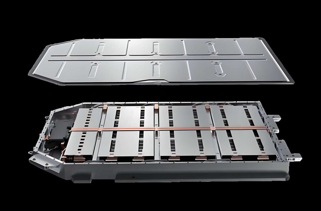
For the analysis in this study, I selected one electric passenger car from the platform and inspected the time-series behavior of its vehicle traction battery over a six-month observation period. The key variables monitored for that vehicle included total pack voltage, total pack current, state-of-charge, maximum cell temperature, minimum cell temperature, vehicle speed, and individual cell voltages. Table 3 summarizes the observed ranges of several important parameters.
| Parameter | Range | Dynamic feature |
|---|---|---|
| Pack voltage (V) | 332.8 – 403.8 | Follows charging and discharging cycles |
| State of charge (SOC) | 29% – 100% | Rapid changes during regenerative braking |
| Max cell temperature (°C) | 11 – 37.5 | Influenced by ambient temperature and load |
| Vehicle speed (km/h) | 0 – 78.8 | Variable driving and parking modes |
| Cell voltage (V) | 3.052 – 4.253 | Strong dependence on SOC and load current |
In the actual cloud data, the operating state of the vehicle traction battery can be divided into four modes based on current and vehicle speed: discharging, charging, resting or sleeping, and offline. When the current is negative and the speed is positive, the vehicle is in the driving-discharge state. When the current is negative and the speed is zero, the vehicle is being charged. When the current is very close to zero and the speed is zero, the vehicle is resting. The offline state occurs when both the current and speed are zero for a long period and the data connection has been temporarily lost. These multiple states increase the difficulty of fault diagnosis because the statistical distribution of the cell voltage is fundamentally different in each state.
Cloud-platform data also contain explicit alarm records. By matching the alarm time with the corresponding battery signals, I examined three illustrative fault events. In the first event, the platform reported a large temperature-difference fault. At the alarm time, one temperature sensor read a value about 6°C higher than the other temperature sensors, while the pack voltage, current, and state-of-charge remained normal. The second event was a discharge-overcurrent fault. The measured current suddenly changed to -43.7 A, which exceeded the designed current limit of the vehicle traction battery. The third event was a cell-temperature anomaly. In that event, the current was only -3.8 A, the pack voltage and SOC were normal, but one temperature reading jumped suddenly and recovered in the next sampling period. The comparison of these events indicates that the first and third events may be caused by sensor malfunction or local thermal inconsistency, while the second event may be caused by an extreme driving condition. This observation guides the design of the fault diagnosis method: different fault types have different statistical signatures in the time series of the vehicle traction battery.
5. Data Preprocessing and Outlier Detection
Raw data collected from the onboard terminal are not directly suitable for mining. Because of communication loss, sensor noise, and intermittent data-logging anomalies, the raw time series of the vehicle traction battery often contain duplicate samples, missing values, and outlier values. Data preprocessing is essential to ensure that the subsequent clustering, statistical diagnosis, and deep-learning prediction operate on reliable samples. My preprocessing workflow includes duplicate removal, missing-data interpolation, and outlier detection.
5.1 Duplicate Removal and Missing-Value Interpolation
In the obtained dataset, some records have the same time stamp as other records. I analyzed ten randomly selected vehicles from the monitoring platform; the number of duplicate samples varied from 0.126% to 0.564% of the total samples. For duplicate records, I retained the first record and removed the redundant ones. The summary statistics are reported in Table 4.
| Vehicle index | Total samples | Duplicate samples | Duplicate rate |
|---|---|---|---|
| Vehicle 1 | 487,505 | 2,207 | 0.45% |
| Vehicle 2 | 548,311 | 2,706 | 0.49% |
| Vehicle 3 | 361,280 | 1,214 | 0.34% |
| Vehicle 4 | 706,832 | 3,406 | 0.48% |
| Vehicle 5 | 202,025 | 254 | 0.13% |
| Vehicle 6 | 140,840 | 209 | 0.15% |
| Vehicle 7 | 746,117 | 4,210 | 0.56% |
| Vehicle 8 | 318,228 | 1,106 | 0.35% |
| Vehicle 9 | 298,268 | 97 | 0.33% |
| Vehicle 10 | 1,048,546 | 4,486 | 0.43% |
For missing data, I applied a continuity check. If the data gap was longer than one minute, I deleted the corresponding segment because interpolation over such a long interval may introduce artificial patterns. If the gap was shorter than one minute, I used cubic-spline interpolation to fill the missing points. Cubic-spline interpolation fits a piecewise cubic polynomial between neighboring known samples and guarantees smoothness and continuity at the connecting points. I prefer cubic-spline interpolation over mean interpolation, weighted-average interpolation, or Lagrange interpolation because it preserves the local trend of the vehicle traction battery signal and avoids the large oscillation often caused by high-order polynomial interpolation.
5.2 Outlier Detection for Different Distribution Types
Outlier detection is applied to remove severe abnormal samples before feature mining. The choice of detection method should depend on the probability distribution of the signal. In the vehicle traction battery, signals such as pack voltage, cell voltage, pack current, and SOC follow an approximately normal distribution when the number of samples is sufficiently large. In this case, I use the 3σ rule. Let the mean of the sampled signal be \(\mu\) and the standard deviation be \(\sigma\). A data point outside the interval
$$ \mu – 3\sigma \le x \le \mu + 3\sigma $$
is regarded as an outlier. The corresponding one-dimensional probability density of a normally distributed signal \(x\) is:
$$ f(x) = \frac{1}{\sqrt{2\pi\sigma^2}} \exp\left[-\frac{(x-\mu)^2}{2\sigma^{2}}\right] $$
For signals that do not follow a normal distribution, such as the frequency of alarms, driving speed, or accumulated driving distance, I use a boxplot-based detection rule rather than the 3σ rule. The boxplot method uses the first quartile \(Q_1\), the median \(Q_2\), and the third quartile \(Q_3\). The interval between the lower and upper fences is
$$ [Q_1 – 1.5\cdot \mathrm{IQR}, \quad Q_3 + 1.5\cdot \mathrm{IQR}] $$
where the interquartile range is defined as:
$$ \mathrm{IQR} = Q_3 – Q_1 $$
Any sample outside this interval is considered a point anomaly. The boxplot method is robust to heavy-tailed distributions and is therefore better suited to non-Gaussian features of the vehicle traction battery fleet data. After preprocessing, the cleaned dataset was used for all later analyses.
6. Dimensionality Reduction and Visualization of Vehicle Traction Battery Voltage Data
The cell voltage matrix of a vehicle traction battery is high-dimensional. For example, a pack with 30 cells in series generates 30 voltage channels at every sampling instant. Real driving data usually produce a very long matrix with strong correlations among the channels. To visualize whether any cell behaves differently from the others, I map all the cell voltages into a two-dimensional space.
Dimensionality reduction methods have different properties. Principal component analysis is a linear method that preserves the global variance of the dataset, but it cannot fully capture nonlinear relationships. Autoencoders can model nonlinear structures but require expensive training and careful tuning. In this study, I selected the t-distributed stochastic neighbor embedding algorithm. This method is efficient in preserving the local distances between neighboring samples, which makes it easy to identify clusters and abnormal separations in the cell-voltage matrix. The t-SNE algorithm is suitable for high-dimensional time-series data generated by the vehicle traction battery because it does not force a linear relationship between cell voltage channels.
After applying t-SNE to the voltage data of one battery pack with 30 cells, the high-dimensional vectors were compressed to two-dimensional scatter points. I observed that most points formed a concentrated cluster, while a small number of points scattered far away from the main cluster. The presence of these distant points indicates that some cells exhibit voltage behavior that deviates from the normal cells. The visualization step alone, however, cannot automatically tell which cell is anomalous. Therefore, I further apply an unsupervised clustering algorithm.
7. Anomaly Detection and Fault Localization of the Vehicle Traction Battery
7.1 K-Means Clustering after t-SNE
For the cleaned voltage dataset after t-SNE dimensionality reduction, I apply the K-means algorithm to divide all points into several clusters. K-means minimizes the within-cluster sum of squared distances:
$$ J = \sum_{j=1}^{K} \sum_{x\in C_j} \|x – \mu_j\|^2 $$
where \(K\) is the number of clusters, \(C_j\) is the set of points in cluster \(j\), and \(\mu_j\) is the centroid of cluster \(j\). A point that lies far from every cluster centroid or belongs to a very small isolated cluster is considered an abnormal voltage point. In the data-mining analysis of the vehicle traction battery, the distance threshold is determined by the formula
$$ P = \mu_d + k \cdot \sigma_d $$
where \(\mu_d\) is the average distance of all data points to their corresponding cluster center, \(\sigma_d\) is the standard deviation of the distance, and \(k\) is a sensitivity coefficient. In the present study I set \(k=1.5\). The clustering results revealed one small isolated cluster and several scattered points that clearly deviated from the main cluster of the vehicle traction battery. These points were marked as abnormal and passed to the next stage for source localization.
7.2 Z-Score Based Fault-Localization Diagnostic Coefficient
To identify which particular cell in the vehicle traction battery produced the abnormal voltage points, I use the Z-score method. Because the actual voltage data are near-normally distributed when enough samples are collected, the probability density of each cell voltage can be expressed by the Gaussian density:
$$ P_i(t) = \frac{1}{\sqrt{2\pi\sigma(t)^2}} \exp\left[-\frac{(V_i(t)-\mu(t))^2}{2\sigma(t)^2}\right] $$
where \(V_i(t)\) is the voltage of cell \(i\) at time \(t\), \(\mu(t)\) is the average of all cell voltages at time \(t\), and \(\sigma(t)\) is the standard deviation of all cell voltages at that time. Then the Z-score of cell \(i\) at time \(t\) is:
$$ Z_i(t) = \frac{V_i(t)-\mu(t)}{\sigma(t)} $$
Since the low probability density value means the cell is far from the normal distribution center, I define an anomaly diagnosis coefficient based on the average probability-density difference of each cell relative to the instantaneous standard deviation:
$$ D_i(t) = \frac{\frac{1}{N}\sum_{i=1}^{N} P_i(t) – P_i(t)}{\sigma_P(t)} $$
where \(N=30\) is the total number of series cells and \(\sigma_P(t)\) is the standard deviation of the probability-density values among all cells. In practice, I calculate the modified Z-index for each cell over the whole time window. A cell with a consistently larger Z-index than the other cells is considered the source of the anomaly.
To validate this approach, I selected a vehicle traction battery pack that was reported to have abnormal voltage fluctuations. Figure-based visual inspection of the raw voltage curves showed that most cells had similar voltage trajectories, but one particular cell, designated as cell 7, had a lower voltage than the other cells and experienced a larger fluctuation. At one moment, the cell-to-cell voltage difference reached 236 mV, and the voltage of cell 7 dropped to about 3.067 V. The calculated Z-values of all 30 cells clearly exhibited the largest deviation for cell 7. Therefore, the combination of K-means clustering and Z-score diagnosis successfully detected the existence of an anomaly in the vehicle traction battery and located the abnormal cell.
8. Comprehensive Performance Evaluation Based on Entropy Weight and Coefficient of Variation
After the faulty cell has been located, it is useful to quantify the severity of the anomaly and to compare the relative state of all cells in the vehicle traction battery. For this purpose, I employ a comprehensive scoring method that combines the entropy-weight method and the coefficient-of-variation method. The entropy method evaluates the information content of each time index: a time point at which the cell voltages are very irregular provides more diagnostic information. The coefficient-of-variation method measures the relative dispersion of the cell voltages. Combining the two methods avoids the one-sidedness of a single weighting rule.
8.1 Building the Voltage Matrix
Let the original voltage matrix of all cells in the vehicle traction battery be represented by \(\mathbf{U}\) with dimensions \(n \times t\), where \(n\) is the number of cells and \(t\) is the number of time instants:
$$ \mathbf{U} = \begin{bmatrix} u_{11} & u_{12} & \cdots & u_{1t} \\ u_{21} & u_{22} & \cdots & u_{2t} \\ \vdots & \vdots & \ddots & \vdots \\ u_{n1} & u_{n2} & \cdots & u_{nt} \end{bmatrix} $$
The element \(u_{ij}\) denotes the voltage of cell \(i\) at time instant \(j\).
8.2 Entropy-Weight Computation
First, I normalize the voltage value of each cell in each time instant by the column sum:
$$ p_{ij} = \frac{u_{ij}}{\sum_{i=1}^{n} u_{ij}}, \quad i=1,\dots,n; \; j=1,\dots,t $$
Then the information entropy of each time instant is:
$$ e_j = -\frac{1}{\ln n} \sum_{i=1}^{n} p_{ij} \ln p_{ij} $$
The entropy-based weight of time instant \(j\) is:
$$ W_j^{(1)} = \frac{1-e_j}{\sum_{j=1}^{t} (1-e_j)} $$
A lower entropy \(e_j\) means that the cell voltages at that time instant are more chaotic or more diverse, and therefore that time instant receives a higher weight.
8.3 Coefficient-of-Variation Weight Computation
For each time instant \(j\), the mean and standard deviation of the voltages across all cells are:
$$ A_j = \frac{1}{n}\sum_{i=1}^{n} u_{ij} $$
$$ S_j = \sqrt{\frac{1}{n}\sum_{i=1}^{n} (u_{ij}-A_j)^2} $$
The coefficient of variation is:
$$ V_j = \frac{S_j}{A_j} $$
and the corresponding coefficient-of-variation weight is:
$$ W_j^{(2)} = \frac{V_j}{\sum_{j=1}^{t} V_j} $$
8.4 Combined Weight and Composite Score
I combine the two weights using an adjustment coefficient \(\alpha\). In this study, \(\alpha\) is set to 0.4:
$$ W_j^{c} = \alpha W_j^{(1)} + (1-\alpha) W_j^{(2)} $$
The composite score of each cell is then calculated as:
$$ S_i = \sum_{j=1}^{t} W_j^{c} u_{ij} $$
To make the score interpretable, I also calculate the theoretical upper and lower score bounds by replacing the voltage value with the maximum or minimum voltage across all cells at every time instant:
$$ S_{\max} = \sum_{j=1}^{t} W_j^{c} u_{\max,j} $$
$$ S_{\min} = \sum_{j=1}^{t} W_j^{c} u_{\min,j} $$
The average score is:
$$ \bar{S} = \frac{1}{n} \sum_{i=1}^{n} S_i $$
For each cell, the deviation from the mean is written as:
$$ \Delta S_i = S_i – \bar{S} $$
If a cell has a much lower composite score and a large negative deviation, its voltage behavior deviates seriously from the average behavior of the vehicle traction battery. The evaluation results for several cells are illustrated by the representative score bounds and deviations reported in Table 5.
| Cell index | Composite score | Upper bound | Lower bound | Score behavior |
|---|---|---|---|---|
| Cell 1 | 0.46549 | 0.46688 | 0.46534 | Normal |
| Cell 3 | 0.56955 | 0.57078 | 0.56941 | Normal |
| Cell 7 | 0.03540 | 0.96200 | 0.03490 | Abnormal |
| Cell 15 | 0.96340 | 0.96363 | 0.96334 | Normal |
| Cell 22 | 0.93894 | 0.93927 | 0.93889 | Normal |
| Cell 23 | 0.92143 | 0.92180 | 0.92139 | Normal |
| Cell 29 | 0.50589 | 0.50725 | 0.50574 | Normal |
From the calculation, cell 7 showed a significantly lower composite score and the largest negative deviation, which matches the earlier localization by the Z-score method. In a further assessment, I compared the score deviation of cell 7 on three different dates within consecutive months. The deviation became larger with time, indicating that the abnormal condition of the cell was progressively worsening. This suggests that the entropy-weight and coefficient-of-variation score is also a useful indicator for tracking the evolution of a vehicle traction battery anomaly.
9. Fault Diagnosis Using the 3σ Multi-Stage Screening Criterion
To obtain a deeper understanding of the fault type and its probability, I developed a fault diagnosis method based on the 3σ multi-stage screening criterion. The conventional 3σ rule has a major drawback: when outliers are present in the data, the calculated mean and standard deviation can be distorted. A single-stage screening process may fail to detect some abnormal cells or may incorrectly label normal cells as outliers. The multi-stage screening process iteratively recalculates the statistical center after excluding abnormal values, thereby producing a more trustworthy center and a narrower normal range for the vehicle traction battery.
9.1 Iterative Screening Algorithm
I formulate the diagnosis process as follows. Let the voltage values of all cells in the vehicle traction battery at time \(t\) be the matrix \(\mathbf{U}^{(0)} = [U_{t,1}^{(0)}, U_{t,2}^{(0)}, …, U_{t,n}^{(0)}]\).
Step 1: Compute the initial mean \(\mu_{t}^{(0)}\) and standard deviation \(\sigma_{t}^{(0)}\) of all cell voltages.
Step 2: Compute the deviation of every cell voltage from the mean:
$$ \Delta V_{i}^{(0)} = V_{i}^{(0)} – \mu_{t}^{(0)} $$
Only those cells satisfying
$$ |\Delta V_{i}^{(0)}| \le 3\sigma_{t}^{(0)} $$
are retained in the new voltage matrix \(\mathbf{U}^{(1)}\). Cells outside this range are temporarily considered as suspected abnormal cells.
Step 3: Using the retained matrix, I compute a new mean \(\mu_{t}^{(1)}\) and a new standard deviation \(\sigma_{t}^{(1)}\), and repeat the screening process. At the \(m\)-th iteration, the retained matrix becomes:
$$ \mathbf{U}^{(m)} = \left\{ V_i^{(m-1)} \; \middle| \; |V_i^{(m-1)}-\mu_t^{(m-1)}| \le 3\sigma_t^{(m-1)} \right\} $$
Step 4: The iterations continue until the convergence condition
$$ |\mu_t^{(m)} – \mu_t^{(m-1)}| < F $$
is satisfied, where \(F\) is a similarity tolerance. In this study, \(F=0.001\). The final center \(\mu_t^{(m)}\) is a robust center of the normal voltage distribution of the vehicle traction battery.
Step 5: After convergence, I define the upper and lower diagnosis thresholds as:
$$ V_{\text{upper}} = \mu_t^{(m)} + \beta \sigma_t^{(m)} $$
$$ V_{\text{lower}} = \mu_t^{(m)} – \beta \sigma_t^{(m)} $$
where \(\beta\) is an empirical coefficient. A cell whose voltage falls outside the interval \([V_{\text{lower}}, V_{\text{upper}}]\) is diagnosed to be in a fault state at time \(t\).
Finally, by extending the process over the complete time window \(T = t_1 \sim t_2\), I obtain a fault matrix \(\mathbf{R}\). If \(r_{ij}=1\), cell \(i\) is in the fault state at time increment \(j\); otherwise \(r_{ij}=0\). The fault probability of cell \(i\) is:
$$ f_i = \frac{1}{T}\sum_{j=1}^{T} r_{ij} \times 100\% $$
9.2 Definition of Systematic Fault and Sudden Fault
Using the fault probability calculated by the 3σ multi-stage criterion, I classified the faults observed in actual vehicles into two general types.
The first type is the systematic fault. This fault arises from the initial inconsistency in materials, cell manufacturing tolerances, or pack design. Its fault probability is low and remains relatively stable over time. In the real-world analysis of the vehicle traction battery, cells of such a pack usually have fault probabilities below 2%, and the faulty cell is often located at a fixed position for a long period. The second type is the sudden fault. This fault arises from an unexpected event such as a temporary internal short circuit, an abnormal discharge current, or a large temperature shock. Its fault probability is usually high, sometimes exceeding 15%, and the location with the highest fault probability can change among different driving cycles. In several vehicle traction battery packs analyzed in this study, most cells had similar probabilities below 2%, but one cell in another pack exhibited a probability of about 17%, which clearly belongs to the sudden-fault category.
10. Comparison of the 3σ-MSS Method with Alternative Outlier-Detection Algorithms
To verify the reliability of the 3σ multi-stage screening diagnosis, I compared it with two widely used outlier-detection algorithms, the connectivity-based outlier factor method and the local outlier factor method. The comparison was performed on the same dataset of the vehicle traction battery under the same preprocessing conditions.
LOF evaluates the local density of each sample relative to its \(k\) nearest neighbors. The reachability distance from \(p\) to \(o\) is defined as:
$$ \text{reach-dist}_k(p,o) = \max\{k\text{-distance}(o), \; d(p,o)\} $$
where \(d(p,o)\) is the Euclidean distance between point \(p\) and point \(o\). The local reachability density of \(p\) is then:
$$ \text{lrd}_k(p) = \frac{|N_k(p)|}{\sum_{o\in N_k(p)} \text{reach-dist}_k(p,o)} $$
and the LOF score is:
$$ \text{LOF}_k(p) = \frac{1}{|N_k(p)|} \sum_{o\in N_k(p)} \frac{\text{lrd}_k(o)}{\text{lrd}_k(p)} $$
A high LOF value means that the point has a much lower density than its neighbors and is likely to be an outlier. COF is similar in spirit to LOF, but it addresses the situation where the data have low-density regions connected by chains; therefore, COF uses the average chaining distance to detect outliers in connected low-density clusters.
The fault probabilities obtained by the three algorithms for the same vehicle traction battery are summarized in Table 6. The COF method produced a much lower maximum fault probability than the other two methods, which indicates that COF may underestimate the fault probability when only a very small number of outlier points are present. The LOF method gave a maximum fault probability that was noticeably higher than that of the 3σ-MSS method, which indicates that LOF may overestimate the fault severity in a dataset with a high proportion of normal points.
| Algorithm | Maximum fault probability | Minimum fault probability | Stability |
|---|---|---|---|
| 3σ-MSS | 0.0213 | 0.0153 | Satisfactory |
| COF | 0.0191 | 0.0040 | Poor at low fault probability |
| LOF | 0.0247 | 0.0143 | Poor at high fault probability |
In the low-probability range, the LOF result and the 3σ-MSS result are close to each other. In the high-probability range, however, LOF tends to produce a larger value and is less stable. COF tends to compress the probability range, making the difference between normal and abnormal cells less obvious. Based on these observations, I conclude that the 3σ-MSS algorithm is the most stable method for the probabilistic diagnosis of cell faults in a vehicle traction battery system.
11. Temporal and Seasonal Fault Probability Analysis of the Vehicle Traction Battery
The cloud platform dataset spans three complete years of operation. To understand how environmental temperature and seasonal climate affect the fault behavior of the vehicle traction battery, I divided the data into four seasonal groups: spring, summer, autumn, and winter. For each season, I calculated the fault probability of every cell in ten vehicles of the same type. The results are summarized in Table 7.
| Season | Maximum single-cell fault probability | Average cell fault probability | Observation |
|---|---|---|---|
| Spring | 1.99% | 1.54% | Lowest overall risk |
| Summer | 4.95% | 4.31% | High temperature increases faults |
| Autumn | 3.67% | 3.07% | Moderate risk |
| Winter | 9.52% | 4.59% | Highest maximum probability |
Both summer and winter show higher average fault probabilities than spring and autumn. This seasonal pattern is related to the operating temperature of the vehicle traction battery. In summer, high ambient temperature accelerates the internal chemical reaction rate and can cause the battery temperature to rise above the optimum range. In winter, low temperature reduces the electrolyte conductivity and may force the battery management system to charge at a high polarization voltage. The risk of lithium plating and local overpotential is increased during cold-weather charging. The vehicle traction battery is therefore most vulnerable to faults when the operating temperature is close to the boundary of its safe window.
I also analyzed the fault probabilities of one vehicle across the three years of data collection with the same 3σ-MSS method. In the first year, the maximum fault probability was about 2.0% on a particular day. Such a low value suggests a systematic inconsistency. In the second year, the maximum fault probability increased to 12.7%, while the average probability of all cells on the same day was about 4.2%. In the third year, the maximum value reached 14.1%, while the average probability was about 3.7%. These results show that with the growth of operation time, some cells of the vehicle traction battery experience a significant increase in fault probability. The fault probability method can therefore be used to follow the long-term degradation trend of individual cells in the vehicle traction battery.
12. Voltage Prediction and Fault Warning of the Vehicle Traction Battery Based on IGWO-CNN-LSTM
The fault diagnosis method described so far can detect, locate, and classify an existing anomaly of the vehicle traction battery. However, to achieve true early warning, it is necessary to predict the future voltage of the cells before the fault alarm threshold is reached. For this reason, I developed a hybrid deep-learning framework based on a convolutional neural network (CNN), a long short-term memory network (LSTM), and an improved grey wolf optimizer (IGWO). The proposed model simultaneously extracts both spatial features and temporal dependencies from the historical data of the vehicle traction battery, and then makes multi-step-ahead voltage predictions.
12.1 Framework of the Prediction Model
The complete prediction process includes the following stages: data import from the cloud platform, data cleaning and feature selection, correlation analysis, feature parameter optimization by the improved grey wolf optimizer, offline training of the CNN-LSTM model, online prediction of future cell voltage, and comparison with alarm thresholds. I trained the model using data from a single vehicle traction battery over a multi-month period and validated the model using data from a different time segment. The model is based on a many-to-one sequence structure: a sliding window of past voltage and auxiliary variables is used as input, and the model outputs the future voltage value.
12.2 Correlation-Based Feature Selection
To select informative inputs, I quantified the correlation of the cell voltage with the pack voltage, pack current, state-of-charge, maximum temperature, minimum temperature, cumulative mileage, and vehicle speed. I used both the Pearson linear correlation coefficient and the Spearman rank correlation coefficient. The Pearson coefficient is calculated as:
$$ \rho = \frac{\sum_{j=1}^{n} (x_j-\bar{x})(y_j-\bar{y})}{\sqrt{\sum_{j=1}^{n} (x_j-\bar{x})^2} \sqrt{\sum_{j=1}^{n} (y_j-\bar{y})^2}} $$
The Spearman coefficient uses the rank values of \(x_j\) and \(y_j\) instead of their raw values:
$$ R_s = 1 – \frac{6\sum d_j^2}{n(n^2-1)} $$
where \(d_j\) is the difference between the ranks of the two variables for observation \(j\). The analysis of the vehicle traction battery data showed that the state-of-charge and the pack total voltage had the strongest correlation with the individual cell voltage. Therefore, I used the previous cell voltage, the total pack voltage, and the state-of-charge as the principal inputs of the deep-learning model.
12.3 Hybrid CNN-LSTM Neural Network
The CNN component contains a one-dimensional convolution layer that extracts local patterns in the input sequence. Let \(\mathbf{x}_{c}^{(l-1)}\) be the output feature map from the \(l-1\)-th layer. The convolution operation followed by batch normalization and a rectified linear unit activation function is represented as:
$$ z_k^{(l)} = \mathrm{ReLU}\left(\sum_{c=1}^{C} \mathbf{W}_{k,c}^{(l)} * \mathbf{x}_{c}^{(l-1)} + b_k^{(l)}\right) $$
where \(\mathbf{W}_{k,c}^{(l)}\) is the convolution kernel, \(b_k^{(l)}\) is the bias term, and \(*\) denotes the convolution operation. The max-pooling operation reduces the dimension of the feature map and retains the most significant high-level features. The features learned by the CNN are flattened and passed to the LSTM layer, which models the temporal dependence.
The LSTM network processes the input sequence by updating the following internal states. At time step \(t\), the forget gate is:
$$ f_t = \sigma\left(W_{xf} x_t + W_{hf} h_{t-1} + b_f\right) $$
The input gate is:
$$ i_t = \sigma\left(W_{xi} x_t + W_{hi} h_{t-1} + b_i\right) $$
The candidate memory cell is:
$$ \tilde{C}_t = \tanh\left(W_{xc} x_t + W_{hc} h_{t-1} + b_c\right) $$
The memory cell is updated as:
$$ C_t = f_t \odot C_{t-1} + i_t \odot \tilde{C}_t $$
The output gate is:
$$ o_t = \sigma\left(W_{xo} x_t + W_{ho} h_{t-1} + b_o\right) $$
The final hidden state is:
$$ h_t = o_t \odot \tanh(C_t) $$
In the hybrid architecture, the CNN layer functions as a feature extractor, while the LSTM layer learns the long-term dependencies in the dynamic voltage signal of the vehicle traction battery. The structural layers are summarized in Table 8.
| Layer function | Configuration | Purpose |
|---|---|---|
| Input layer | Sequence of voltage-related features | Load the normalized time-series samples |
| Convolution layer | Several one-dimensional filters | Extract local spatial features |
| Batch normalization | Channel-wise normalization | Stabilize the training and reduce internal covariate shift |
| Activation layer | ReLU | Add nonlinearity |
| Max pooling | Down-sampling | Reduce feature dimension and preserve important attributes |
| Flatten layer | Reshape feature maps | Bridge between CNN and LSTM |
| LSTM layer | Memory cells with gates | Model long-term temporal dependencies |
| ReLU layer | After LSTM | Improve the representation ability |
| Fully connected layer | Dense output | Map the extracted features to the predicted voltage |
| Regression output | Mean-square error loss | Train for quantitative voltage prediction |
12.4 Improved Grey Wolf Optimizer for Hyper-Parameter Optimization
The architecture of the CNN-LSTM model contains a number of hyper-parameters, such as the number of convolution kernels, the pooling size, and the number of LSTM hidden units. An improper selection of these hyper-parameters can strongly degrade the prediction accuracy. I therefore implemented an improved grey wolf optimizer to search for the optimal hyper-parameters.
In the standard grey wolf optimizer, the pack of grey wolves is divided into alpha, beta, delta, and omega individuals. During the hunting process, the position update of a grey wolf is formulated as:
$$ \vec{D} = |\vec{C}\cdot\vec{X}_p(t) – \vec{X}(t)| $$
$$ \vec{X}(t+1) = \vec{X}_p(t) – \vec{A}\cdot\vec{D} $$
The coefficient vectors are:
$$ \vec{A} = 2\vec{a}\cdot\vec{r}_1 – \vec{a} $$
$$ \vec{C} = 2\cdot\vec{r}_2 $$
where \(\vec{r}_1\) and \(\vec{r}_2\) are random vectors in \([0,1]\). In the standard algorithm, the convergence factor \(\vec{a}\) decreases linearly from 2 to 0 as the iterations proceed. In the improved grey wolf optimizer, I introduce a nonlinear adjustment of the convergence factor, and I apply a Cauchy mutation operation to the candidate positions. The mutation perturbs the wolf positions by a random value drawn from the Cauchy distribution after the main position update, which helps the algorithm escape from local optima and improves the global search capability during the optimization of the vehicle traction battery prediction model.
The mean square error between the predicted voltage and the actual voltage is used as the fitness function:
$$ \text{Loss}(\theta) = \frac{1}{n}\sum_{i=1}^{n} \left( \hat{u}_i – u_i \right)^2 $$
where \(u_i\) is the measured voltage and \(\hat{u}_i\) is the predicted voltage. The improved grey wolf optimizer searches for the model parameters \(\theta\) that minimize this loss.
12.5 Evaluation Metrics
I evaluate the prediction accuracy using the mean absolute error, root mean square error, and coefficient of determination. These metrics are defined as:
$$ \mathrm{MAE} = \frac{1}{n}\sum_{i=1}^{n} |\hat{u}_i – u_i| $$
$$ \mathrm{RMSE} = \sqrt{\frac{1}{n}\sum_{i=1}^{n} (\hat{u}_i – u_i)^2} $$
$$ R^2 = 1 – \frac{\sum_{i=1}^{n}(\hat{u}_i-u_i)^2}{\sum_{i=1}^{n}(u_i-\bar{u})^2} $$
Smaller MAE and RMSE values indicate better prediction accuracy, while an \(R^2\) value closer to one indicates a better fitting performance.
12.6 Comparison of Different Models
Using the same dataset containing the vehicle traction battery operating data, I trained five models: BiLSTM, LSTM, CNN-LSTM, CNN-GRU, and IGWO-CNN-LSTM. In the comparison, all models used the same input window, the same preprocessing procedure, and the same evaluation strategy. The objective is to isolate the effect of the network structure and the optimizer. I first compared the CNN-LSTM model with the IGWO-CNN-LSTM model. The CNN-LSTM model without hyper-parameter optimization produced a maximum absolute voltage error of about 30 mV, whereas the IGWO-CNN-LSTM model reduced this maximum error to about 24 mV. This demonstrates that the improved grey wolf optimizer successfully improves the generalization capability of the model.
| Model | MAE (mV) | MAPE (%) | RMSE (mV) | \(R^2\) |
|---|---|---|---|---|
| BiLSTM | 7.3997 | 0.18962 | 9.6738 | 0.99647 |
| LSTM | 9.1646 | 0.23348 | 11.5940 | 0.99493 |
| CNN-LSTM | 6.2004 | 0.16033 | 8.4264 | 0.99732 |
| CNN-GRU | 4.4459 | 0.11321 | 5.4142 | 0.99889 |
| IGWO-CNN-LSTM | 3.5254 | 0.09009 | 4.5086 | 0.99923 |
The results in Table 9 show that the proposed IGWO-CNN-LSTM model achieves the lowest MAE, RMSE, and MAPE, and the highest \(R^2\) value. Compared with the LSTM model, the MAE is reduced by more than 60%, and the RMSE is reduced from 11.594 mV to 4.509 mV. Compared with CNN-LSTM, the RMSE is reduced from 8.426 mV to 4.509 mV. The improvement is particularly important for the vehicle traction battery because even a small voltage prediction error may affect the reliability of the warning threshold.
12.7 Validation of Fault Prediction
After the model was trained and validated, I tested whether the predicted voltage could provide early warnings when the actual cell voltage later exceeded the overvoltage threshold. A segment of data was extracted from a vehicle traction battery record that included a voltage anomaly. A sliding window of historical samples was used as model input, and the future voltage trajectory was predicted. I defined an alarm threshold at 4.3 V for the examined battery. In the interval between sampling points 4480 and 4500, the measured cell voltage exceeded 4.3 V. The predicted voltage based on earlier samples exceeded the threshold at an earlier time, thus anticipating the actual overvoltage event by roughly one minute. The result suggests that the proposed deep-learning method is capable of predicting the abnormal voltage trend of the vehicle traction battery before the fault occurs.
13. Fault Warning Strategy and Maintenance Recommendations
Predicted voltage values are useful for early warning only when connected to an appropriate set of warning rules. In this study, I integrated four voltage-related fault categories for the vehicle traction battery: overvoltage, undervoltage, fast voltage rise-rate, fast voltage fall-rate, and inconsistency among cells. The former two categories indicate that the cell voltage exceeds its safety window. The latter two categories capture dynamical abnormal changes of the voltage. The cell-to-cell voltage inconsistency is measured by the instantaneous standard deviation of all cell voltages.
| Fault type | Classification criterion | Warning interpretation |
|---|---|---|
| Cell overvoltage | \(4.3\ \mathrm{V} \le U \le 4.8\ \mathrm{V}\) | Potential overcharge; minor warning |
| Severe cell overvoltage | \(U > 4.8\ \mathrm{V}\) | Serious overcharge; immediate action |
| Cell undervoltage | \(U \le 3.4\ \mathrm{V}\) | Deep discharge; dangerous state |
| Rapid voltage rise | \(\Delta U \ge 0.4\ \mathrm{V/s}\) | Severe charging abnormal |
| Rapid voltage drop | \(\Delta U \le -0.4\ \mathrm{V/s}\) | Potential internal short circuit |
| Cell inconsistency | \(\sigma \ge 0.5\ \mathrm{V}\) among cell voltages | Poor consistency; capacity limitation needed |
In my warning strategy, the levels are defined according to the severity of the operation risk. A level-1 warning indicates the most severe state, for example an undervoltage fault, a rapid voltage change, or a large cell inconsistency. The driver should immediately stop the vehicle and cut off the high-voltage system. A level-2 warning indicates that the vehicle traction battery has reached a dangerous threshold, such as an overvoltage above the absolute maximum limit. The vehicle should be stopped and inspected as soon as possible. A level-3 warning indicates that a slight but noticeable deviation has been identified, such as the cell voltage entering the early overvoltage zone. The driver should schedule a maintenance check, reduce the charging current limit, and carefully observe whether the voltage anomaly grows with time.
From the perspective of operation and maintenance, the following recommendations are useful. First, for a sudden-fault battery, the vehicle should be kept under observation and the abnormal module should be replaced as soon as possible. Second, for a systematic fault caused by fixed cell inconsistency, cell balancing and careful charging management are more appropriate. Third, seasonal influences should be considered: in summer, the thermal-management system should be checked to avoid overheating of the vehicle traction battery; in winter, charging should preferably be performed with a warmed battery or at a reduced current to avoid lithium plating. Fourth, when the predicted voltage of a cell follows a continuously worsening trend, a module-level inspection should be arranged even if no warning threshold has been exceeded. The combination of 3σ-MSS fault probability diagnosis and IGWO-CNN-LSTM voltage prediction therefore gives a practical, scalable, and proactive tool for maintaining the safety of the vehicle traction battery.
14. Discussion
The results of this study demonstrate that the vehicle traction battery state can be efficiently monitored through the integration of statistics and deep learning. The proposed framework has several advantages for actual electric-vehicle fleets. First, the method does not require a physical battery model. The entire diagnosis is based on the data collected by the mandatory cloud-monitoring platform. This makes the framework easy to deploy for millions of vehicles. Second, the multi-level screening method is robust against the dynamic operating conditions of the vehicle traction battery. Because the screening procedure recalculates the statistical center in an iterative way, it can identify cells that deviate from the main voltage pattern even if the whole pack voltage changes with speed, acceleration, or state-of-charge. Third, the entropy-weight combined score gives a physical ranking of the severity of all cells. This ranking is very useful for deciding which module of the vehicle traction battery should be inspected first. Fourth, the CNN-LSTM voltage-prediction model makes use of the temporal context of the data. It not only detects the current fault but also predicts the future voltage behavior, which makes real early warning possible.
Nevertheless, there are limitations in the present study. The cloud-platform data do not include the exact internal physical state of every cell. Thus, the relation between the diagnosed voltage anomaly and the true internal mechanism of the vehicle traction battery is inferred indirectly. Furthermore, the selection of warning thresholds depends on the specific chemistry and design of a given vehicle traction battery. It is necessary to calibrate the thresholds under laboratory conditions or to use manufacturer specifications. Finally, the current deep-learning model was optimized for one specific driving dataset; transferring the model to another vehicle type may require extra training or additional adaptation data.
15. Conclusion and Future Work
In this work, I carried out a systematic study on anomaly detection, fault localization, fault diagnosis, and voltage prediction of the vehicle traction battery based on a large real-world operating dataset. The main conclusions of this study are as follows.
First, the raw cloud-platform data of the vehicle traction battery contain repeated records, missing points, and outliers. The quality of the data can be significantly improved by removing the duplicate samples, interpolating short gaps with the cubic-spline method, and applying the 3σ rule for approximately normally distributed variables or the boxplot rule for non-Gaussian variables.
Second, the t-SNE visualization followed by K-means clustering provides a useful way to detect anomalous cells in the multidimensional voltage matrix of the vehicle traction battery. The Z-score-based diagnostic coefficient is able to locate the abnormal cell with relatively high confidence. In the case study, one particular cell was found to have a much larger Z-index than all other cells and was subsequently identified as the fault source.
Third, the entropy-weight combined coefficient-of-variation method gives a comprehensive score for each cell. This score not only detects an abnormal cell but also evaluates its degree of deviation. Repeated calculation of the score over time revealed that the score deviation of the faulty cell increased, which proves that the method is useful for tracking the progression of a fault in the vehicle traction battery.
Fourth, the 3σ multi-stage screening method outperforms both COF and LOF in the fault probability analysis of the vehicle traction battery. It provides stable fault probabilities for both low-probability systematic faults and high-probability sudden faults. Seasonal analysis of the data over three years indicates that summer and winter create more severe fault risks for the vehicle traction battery than spring and autumn.
Fifth, the hybrid IGWO-CNN-LSTM model was developed for multi-step voltage prediction of the vehicle traction battery. The proposed model achieved the best prediction performance among all compared models, with an MAE of 3.5254 mV and an RMSE of 4.5086 mV. This prediction accuracy is sufficient to detect the trend toward an overvoltage or undervoltage fault. Combined with a practical warning strategy, the model can warn the driver about the future state of the vehicle traction battery with enough lead time to avoid severe consequences.
In future work, I plan to test the proposed algorithm on a larger heterogeneous fleet of electric vehicles and to incorporate more failure labels such as actual thermal runaway records into the training process. I also intend to investigate multi-fault joint diagnosis of the vehicle traction battery, where different faults occur simultaneously or sequentially. The deep-learning model can be further improved by adding attention mechanisms and by using transfer learning to adapt the model to different vehicle models without collecting a large amount of labeled data. Finally, the ultimate research goal is to build an online, cloud-native safety-monitoring engine for the vehicle traction battery in which each individual cell is evaluated, tracked, and warned in real time, thus improving the safety and reliability of electric vehicles at a fleet level.