
At ROTDYN2022, I presented two investigations that at first appear to be unrelated to one another. The first investigation is concerned with the vibration response of a helicopter tail horizontal shaft with an end-tooth folding mechanism. The second investigation is concerned with fault diagnosis of the regenerative braking system in an electric car. When these two subjects are viewed through the common lens of rotor dynamics, their connection becomes clear. Both involve rotating components, nonlinear interactions between mechanical and electrical parts, and the need to interpret measured or predicted dynamic responses accurately. The helicopter tail shaft transmits power through a folding mechanism that contains spline joints and end teeth. The electric car contains a drive motor, reduction gear, half-shafts, and wheels that exchange kinetic energy during regenerative braking. In both cases, the engineer needs reliable models and decision tools to avoid unexpected vibration, fatigue, or failure.
Throughout this article, I use the phrase “electric car” deliberately. The electric car is not merely a vehicle with a battery and motor; it is also a rich source of dynamic signals. During regenerative braking, an electric car uses its traction motor as a generator. The motor applies a negative torque to the driven wheels and converts the kinetic energy of the moving electric car into electrical energy that is stored in the battery. This operation is highly coupled with the electrical state of the battery, the mechanical state of the brake system, and the instantaneous speed of the rotating drivetrain. Therefore, the fault diagnosis of an electric car’s regenerative braking system is a perfect example of the complex nonlinear problems that can be treated with modern machine-learning algorithms.
1. Motivation and Engineering Context
The first motivation for the helicopter part of my work is closely related to carrier-based operation. The number of helicopters that can be parked on a carrier deck is always limited by the available floor area. If the tail part of a helicopter can be folded, the footprint of each helicopter is reduced, and more helicopters can be accommodated in the same area. The tail horizontal shaft is one of the components that has to be folded and unfolded repeatedly. A folding mechanism with end teeth can provide a compact and reliable way to disconnect and reconnect the shaft. However, during service, the folded shaft is not a simple continuous beam. The spline connection and end-tooth connection introduce local flexibility that cannot be ignored. If the tail horizontal shaft is modeled as a rigid continuous shaft, the vibration response at the supports may be incorrect. I therefore chose to construct a dynamic model that explicitly represents the stiffness discontinuities associated with the folding mechanism.
The second motivation is the safety and efficiency of the regenerative braking process in an electric car. An electric car brakes not only by friction but also by regenerative torque. If the regenerative braking controller receives a large braking demand while the battery is almost fully charged, the controller must limit the regenerative torque and increase the friction torque. This switching process introduces nonlinearity and abrupt changes in torque. If a sensor or actuator fails, the braking behavior of the electric car can become unsafe. Such faults are difficult to identify because the measured data have high dimensions and strong nonlinear correlations. In my work, I used kernel principal component analysis, abbreviated KPCA, to reduce these high-dimensional nonlinear data, and then used a support vector machine, abbreviated SVM, to classify the fault modes of the electric car. I also used firefly algorithm to optimize the parameters of the KPCA and SVM models. The result was a fault-diagnosis method that is both accurate and suitable for the complex operation of an electric car.
2. Vibration Response of a Helicopter Tail Horizontal Shaft with an End-Tooth Folding Mechanism
In this part of my study, I considered a helicopter tail horizontal shaft that contains a folding mechanism. The role of this shaft is to transmit mechanical power from the main gearbox area toward the tail rotor. When the required landing space is reduced, the shaft must be folded. The folding mechanism uses two important load-carrying connections: a spline connection and an end-tooth connection. To predict the vibration response accurately, I first decomposed the folding mechanism into simpler structural elements. The spline connection was treated as an elastic joint with radial stiffness and angular stiffness. The end-tooth connection was represented by an equivalent ring. This simplification allowed the detailed tooth geometry to be removed from the finite element model while retaining the important stiffness and mass effects.
2.1 Equivalent Description of the Spline Connection
Let the degree-of-freedom vectors at two adjacent nodes of the finite element model be denoted by \(\mathbf{q}_A\) and \(\mathbf{q}_B\). In a general spatial shaft model, each node has translational and rotational degrees of freedom. The vector can be written as
\[
\mathbf{q} = [u, v, w, \theta_x, \theta_y, \theta_z]^T,
\]
where \(u, v, w\) are translations and \(\theta_x, \theta_y, \theta_z\) are rotations about the global coordinate axes. For a spline connection, the relative displacement between the two nodes is
\[
\Delta \mathbf{q} = \mathbf{q}_B – \mathbf{q}_A.
\]
The strain energy stored in the equivalent spline element is represented by
\[
U_s = \frac{1}{2} (\mathbf{q}_B – \mathbf{q}_A)^T \mathbf{K}_s (\mathbf{q}_B – \mathbf{q}_A),
\]
where \(\mathbf{K}_s\) is the equivalent stiffness matrix of the spline connection. In my modeling approach, the dominant terms in \(\mathbf{K}_s\) are the radial stiffness \(k_r\) and the angular stiffness \(k_\theta\). The radial stiffness acts against relative lateral displacements between the two shaft segments, while the angular stiffness acts against relative bending rotations. The physical meaning of the spline connection is therefore retained without modeling every individual spline tooth. This reduces the computational size of the finite element model and improves numerical efficiency. The basic equivalent components are summarized in Table 1.
| Component | Equivalent structural element | Primary stiffness terms | Reason for simplification |
|---|---|---|---|
| Spline connection | Spring-like elastic joint | Radial stiffness \(k_r\), angular stiffness \(k_\theta\) | Detailed spline teeth are too small for global shaft model |
| End-tooth connection | Equivalent ring element | Bending stiffness \(EI_{eq}\), distributed mass \(\rho A_{eq}\) | Tooth ring acts as a continuous annular structure when fully engaged |
In the table, the notation \(EI_{eq}\) denotes the equivalent flexural stiffness of the ring and \(\rho A_{eq}\) denotes the equivalent mass per unit length. The actual tooth ring is not perfectly uniform, but the equivalent ring model gives a good representation of the overall bending and inertial behavior in the low- and medium-frequency range.
2.2 Equivalent Representation of the End-Tooth Connection
The end-tooth connection is another important part of the folding mechanism. When the folding mechanism is assembled, the end teeth of the two coupling halves engage with each other. The tooth ring has a complex geometry, but the main dynamic contribution of this joint is its bending stiffness and inertia. In my finite element model, I therefore replaced the end-tooth connection with an equivalent ring. The equivalent ring is a short annular beam with a circular cross-section of outer diameter \(D_o\) and inner diameter \(D_i\). The equivalent cross-sectional area and second moment of area are
\[
A_{eq} = \frac{\pi}{4}(D_o^2 – D_i^2),
\]
\[
I_{eq} = \frac{\pi}{64}(D_o^4 – D_i^4).
\]
If the original tooth ring contains several disconnected tooth segments, the equivalent Young’s modulus can be adjusted so that the bending stiffness of the ring matches the bending stiffness of the real tooth connection. The equivalent stiffness is written as
\[
EI_{eq} = E_{eq} I_{eq}.
\]
Similarly, the equivalent distributed inertia is written as
\[
\rho A_{eq} = \rho_{eq} A_{eq}.
\]
By using a ring model, I avoided the need to generate a very fine three-dimensional mesh of the teeth in every global shaft vibration analysis. The equivalent ring therefore serves as a bridge between detailed local finite element analysis and the overall system dynamic model.
2.3 Lumped-Mass Dynamic Model of the Tail Horizontal Shaft
After equivalent finite element matrices were constructed, I reduced the mechanical model with a concentrated mass approach. This lumped-mass method is common in rotor-dynamics studies because it enables a compact representation of the shaft, supports, couplings, and attachments. The spatial model of the complete tail horizontal shaft is written as
\[
\mathbf{M} \ddot{\mathbf{r}}(t) + \left[ \mathbf{C} + \Omega \mathbf{G} \right] \dot{\mathbf{r}}(t) + \mathbf{K} \mathbf{r}(t) = \mathbf{f}(t),
\]
where \(\mathbf{M}\) is the mass matrix, \(\mathbf{C}\) is the damping matrix, \(\mathbf{G}\) is the gyroscopic matrix, \(\Omega\) is the rotational speed, \(\mathbf{K}\) is the total stiffness matrix, \(\mathbf{r}(t)\) is the vector of generalized coordinates, and \(\mathbf{f}(t)\) is the external force vector. The gyroscopic matrix is important when the rotor speed is high and the forward and backward whirl motions differ.
The correctness of the model was first checked by calculating the critical speeds. For free vibration of the undamped rotating shaft, the homogeneous equation is
\[
\mathbf{M} \ddot{\boldsymbol{\phi}}(t) + \Omega \mathbf{G} \dot{\boldsymbol{\phi}}(t) + \mathbf{K} \boldsymbol{\phi}(t) = \mathbf{0}.
\]
Assuming a harmonic solution of the form
\[
\boldsymbol{\phi}(t) = \boldsymbol{\Phi} e^{j \omega t},
\]
the eigenvalue problem becomes
\[
\left[ – \omega^2 \mathbf{M} + j \omega \Omega \mathbf{G} + \mathbf{K} \right] \boldsymbol{\Phi} = \mathbf{0}.
\]
For a given rotational speed \(\Omega\), the natural frequencies of the forward and backward modes can be found. A critical speed occurs when one of the system natural frequencies coincides with an excitation harmonic of the shaft. For a conventional rotating shaft with unbalance excitation, the excitation order is the first order, so
\[
\omega = \Omega.
\]
For the folded tail horizontal shaft, I considered both the folded state and the unfolded state. The critical-speed calculation was used as a verification step because the predicted critical speeds must remain continuous when the model is refined. Once the model was accepted, the next step was to compute the time-domain vibration response of the shaft supports.
2.4 Time-Domain Solution Using the Newmark Method
The support response of the tail horizontal shaft under unbalance and other excitation forces depends strongly on the transient behavior of the system. I used the Newmark time integration method to solve the second-order differential equations. In the Newmark method, the recurrence equations for displacement and velocity are
\[
\mathbf{r}_{n+1} = \mathbf{r}_n + \Delta t \dot{\mathbf{r}}_n + \left( \frac{1}{2} – \beta \right) \Delta t^2 \ddot{\mathbf{r}}_n + \beta \Delta t^2 \ddot{\mathbf{r}}_{n+1},
\]
\[
\dot{\mathbf{r}}_{n+1} = \dot{\mathbf{r}}_n + (1 – \gamma) \Delta t \ddot{\mathbf{r}}_n + \gamma \Delta t \ddot{\mathbf{r}}_{n+1}.
\]
The constants \(\beta\) and \(\gamma\) determine the accuracy and stability of the method. In many rotor-dynamics applications, I choose
\[
\beta = \frac{1}{4}, \qquad \gamma = \frac{1}{2},
\]
which corresponds to the constant-average-acceleration method and is unconditionally stable for linear systems. At every time step, the equivalent stiffness matrix can be written as
\[
\mathbf{K}_{\mathrm{eff}} = \mathbf{K} + \frac{1}{\beta \Delta t^2} \mathbf{M} + \frac{\gamma}{\beta \Delta t} \left[ \mathbf{C} + \Omega \mathbf{G} \right].
\]
The equivalent force vector at the new time step depends on the external load, the damping matrix, and the previous displacement, velocity, and acceleration vectors. Solving this recurrence relation gives the vibration response of every node on the shaft. From the nodal response, I extracted the vibration displacement and forces at the support bearings. The method allowed me to compare how the folding mechanism changes the support vibration relative to a straight continuous shaft.
In a practical tail shaft dynamic analysis, the most important excitation is often the unbalance force generated by a small mass eccentricity \(e\) on the rotating part. For a concentrated unbalance mass \(m_d\) located at a node, the force components can be expressed as
\[
f_x(t) = m_d e \Omega^2 \cos(\Omega t),
\]
\[
f_y(t) = m_d e \Omega^2 \sin(\Omega t).
\]
The response at any support bearing is then determined from the displacement history of the corresponding node. The equivalent radial bearing force can be computed as
\[
\mathbf{F}_{\mathrm{support}}(t) = \mathbf{K}_b \mathbf{r}_b(t) + \mathbf{C}_b \dot{\mathbf{r}}_b(t),
\]
where \(\mathbf{K}_b\) and \(\mathbf{C}_b\) are the bearing stiffness and damping matrices, and \(\mathbf{r}_b(t)\) is the displacement vector at the bearing location. This gave me a clear picture of the vibration level that the folding joint produces during operation.
The main contributions of this first part of my work are therefore the modeling strategy for the spline connection and end-tooth connection and the use of a lumped-mass dynamic model for the full assembly. The technique of replacing complicated teeth with equivalent stiffness and equivalent ring elements is useful because it creates a lightweight model that still retains the physical effect of the folding mechanism on the overall vibration response.
3. FA-Optimized KPCA-SVM Fault Diagnosis for a Regenerative Braking System in an Electric Car
The second part of my work was devoted to the diagnosis of faults in the regenerative braking system of an electric car. This topic is especially interesting because the rotating drivetrain of an electric car is not isolated from the electrical system. The electric car is a complex machine in which a mechanical braking action can affect motor current, battery state of charge, wheel slip, and vehicle deceleration simultaneously.
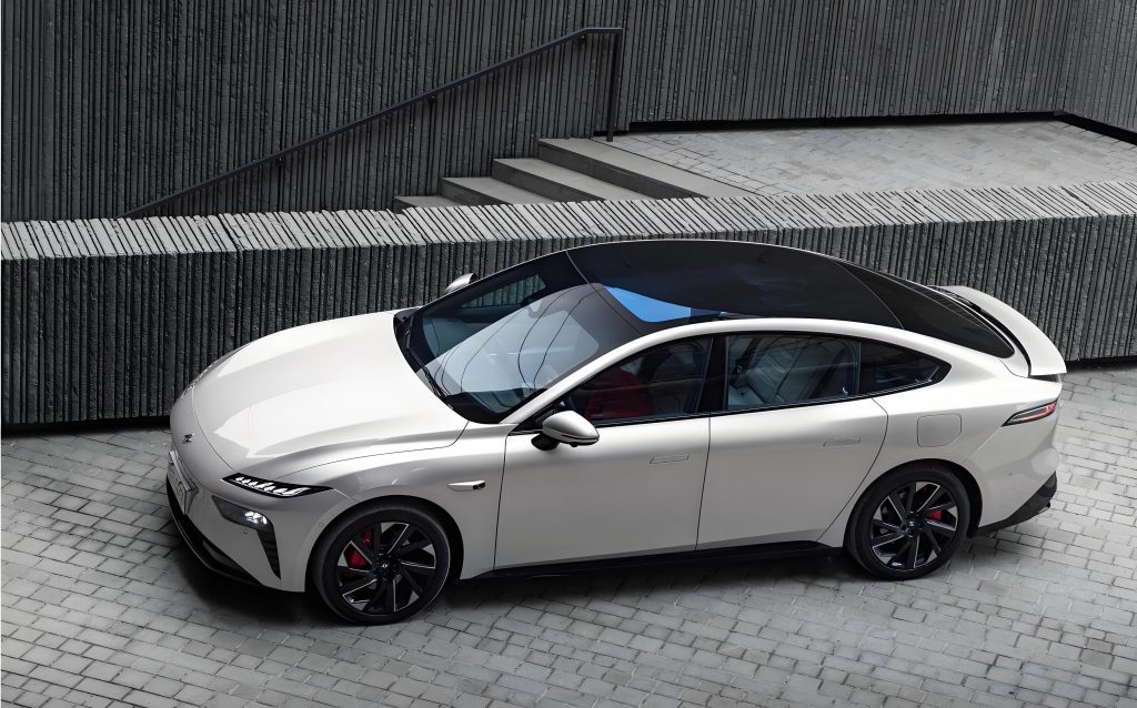
Regenerative braking is a central function in every electric car that is used for energy saving. When the driver of an electric car presses the brake pedal, the vehicle controller calculates the total braking torque demand. This total demand is split between the regenerative braking torque produced by the motor and the friction braking torque produced by the hydraulic brake system. The regenerative torque is limited by the maximum motor torque and by the maximum charging current that the battery can accept. Therefore, the operation of the electric car depends strongly on the motor speed, temperature, battery voltage, and battery state of charge. Any fault in these components can cause an incorrect torque distribution and reduce the braking safety of the electric car.
In an electric car, measured data have several special properties. First, the signals are high-dimensional because many sensors are installed in the motor controller, battery management system, and hydraulic brake unit. Second, the signals are nonlinear because the regenerative torque limit changes with the battery state of charge. Third, the signals are highly correlated because the motor current, voltage, torque, and vehicle deceleration all respond to the same braking demand. Linear fault-diagnosis methods often fail when applied directly to such data. For this reason, I used KPCA to project the original data into a high-dimensional feature space where nonlinear relationships become linear enough to be analyzed.
3.1 Kernel Principal Component Analysis
Suppose that the original data sample collected from an electric car is represented by a vector \(\mathbf{x}_i \in \mathbb{R}^m\). A nonlinear feature mapping is defined as
\[
\Phi: \mathbb{R}^m \rightarrow \mathcal{F},
\]
where \(\mathcal{F}\) is a high-dimensional feature space. Kernel principal component analysis avoids an explicit calculation of the mapping function by using a kernel function. In my analysis, I used the Gaussian radial basis function kernel
\[
k(\mathbf{x}_i, \mathbf{x}_j) = \exp \left( – \frac{\Vert \mathbf{x}_i – \mathbf{x}_j \Vert^2}{2 \sigma^2} \right),
\]
where \(\sigma\) is the kernel width. Let
\[
K_{ij} = k(\mathbf{x}_i, \mathbf{x}_j).
\]
The centered kernel matrix is given by
\[
\widetilde{\mathbf{K}} = \mathbf{K} – \mathbf{1}_N \mathbf{K} – \mathbf{K} \mathbf{1}_N + \mathbf{1}_N \mathbf{K} \mathbf{1}_N,
\]
where \(\mathbf{1}_N\) is an \(N \times N\) matrix with all entries equal to \(1/N\). The eigenvectors of the centered kernel matrix solve the eigenvalue problem
\[
N \lambda_k \alpha_k = \widetilde{\mathbf{K}} \alpha_k.
\]
The score of the \(k\)-th principal component for a new sample \(\mathbf{x}\) is then
\[
t_k(\mathbf{x}) = \sum_{i=1}^{N} \alpha_{k i} k(\mathbf{x}_i, \mathbf{x}).
\]
In this way, the original nonlinear data of the electric car are represented by a smaller set of feature variables \(t_k\). These feature variables are then used to construct monitoring statistics.
3.2 Monitoring Statistics for Fault Detection
After KPCA is applied, I used two standard statistics to monitor the health of the regenerative braking system in an electric car. The first statistic is the Hotelling \(T^2\) statistic. For a retained set of \(p\) principal components, the \(T^2\) statistic is defined as
\[
T^2 = \sum_{k=1}^{p} \frac{t_k^2}{\lambda_k},
\]
where \(\lambda_k\) is the eigenvalue associated with the \(k\)-th principal component. The second statistic is the squared prediction error
\[
\mathrm{SPE} = \sum_{i=1}^{N} t_i^2 – \sum_{k=1}^{p} t_k^2.
\]
If the \(T^2\) or SPE value exceeds the confidence limit of the model, a fault is considered to be present in the regenerative braking system. This monitoring stage is important for distinguishing normal operation from abnormal operation of the electric car. The use of KPCA allows the monitoring model to capture nonlinear relationships that linear PCA would miss.
Table 2 summarizes the variables that are commonly relevant when collecting regenerative braking data from an electric car. These variables are not all independent; they interact with one another through the control strategy of the braking system.
| Variable group | Typical variable | Physical meaning |
|---|---|---|
| Vehicle dynamics | Vehicle speed | Determines the kinetic energy available for regeneration |
| Electric motor | Motor speed and torque | Produces regenerative braking torque in an electric car |
| Battery system | Battery current, voltage, state of charge | Limits the amount of energy that can be recovered |
| Brake system | Brake pedal angle and hydraulic pressure | Indicates driver demand and hydraulic response |
| Control signal | Torque command and regenerative braking command | Shows the desired behavior of the electric car controller |
3.3 Firefly Algorithm for Parameter Optimization
The performance of KPCA depends strongly on the selection of the kernel parameter \(\sigma\). If \(\sigma\) is too small, the model can become too sensitive to noise. If \(\sigma\) is too large, the nonlinear structure of the electric car data may be smoothed away. I therefore applied the firefly algorithm to optimize the kernel parameters of the KPCA model and the SVM classifier. The optimization target was the fault-diagnosis accuracy on the training data.
In the firefly algorithm, each firefly represents one candidate parameter vector. A firefly with better objective function has a higher light intensity and attracts other fireflies. The attractiveness between firefly \(i\) and firefly \(j\) depends on the distance \(r_{ij}\),
\[
r_{ij} = \Vert \mathbf{x}_i – \mathbf{x}_j \Vert.
\]
The attractiveness function is defined as
\[
\beta(r) = \beta_0 e^{- \gamma r^2},
\]
where \(\beta_0\) is the attractiveness at zero distance and \(\gamma\) is a light absorption coefficient. The movement of firefly \(i\) toward firefly \(j\) is updated by the formula
\[
\mathbf{x}_i^{t+1} = \mathbf{x}_i^t + \beta_0 e^{- \gamma r_{ij}^2} (\mathbf{x}_j^t – \mathbf{x}_i^t) + \alpha \left( \mathrm{rand} – \frac{1}{2} \right),
\]
where \(\alpha\) controls the random step size. In the optimization model, the firefly position vector contains the KPCA kernel parameter and the SVM penalty and kernel parameters. Let the candidate parameter vector be
\[
\mathbf{p} = [\sigma_{\mathrm{KPCA}}, \sigma_{\mathrm{SVM}}, C]^T.
\]
The objective function is the cross-validation accuracy of the combined fault-diagnosis model,
\[
\max_{\mathbf{p}} \; A_{\mathrm{CV}}(\mathbf{p}) = \frac{N_{\mathrm{correct}}}{N_{\mathrm{total}}} \times 100\%.
\]
After iterative optimization, the best parameter set was selected for the final KPCA-SVM model. The FA optimization improved the fault-diagnosis accuracy of an electric car regenerative braking system by selecting parameters that adapt to the nonlinear distribution of the data.
3.4 Multi-Class SVM Classification
The support vector machine is originally a binary classifier. For fault diagnosis of an electric car, however, there are usually several fault categories. I therefore compared two ways of extending the binary SVM to multi-class classification. The first approach is called one-versus-one. In this approach, a separate SVM is trained for every pair of classes. If the total number of classes is \(N_c\), the number of binary classifiers is
\[
N_{\mathrm{OVO}} = \frac{N_c (N_c – 1)}{2}.
\]
During classification, every binary classifier makes a decision and the final class is selected by voting. This voting decision is written as
\[
\hat{y} = \arg \max_{c} \; V_c(\mathbf{x}),
\]
where \(V_c(\mathbf{x})\) is the number of binary classifiers that assign the sample to class \(c\). The second approach is called one-versus-all. In this approach, one SVM is trained for each class against all other classes. The final class is the class whose corresponding classifier produces the largest decision function value.
The basic mathematical formulation of a binary SVM is stated as follows. Given a training data set
\[
(\mathbf{x}_i, y_i), \qquad i = 1, 2, \dots, n,
\]
where \(y_i \in \{-1, +1\}\), the optimal separating hyperplane is found by solving
\[
\min_{\mathbf{w}, b, \boldsymbol{\xi}} \; \frac{1}{2} \Vert \mathbf{w} \Vert^2 + C \sum_{i=1}^{n} \xi_i,
\]
subject to
\[
y_i \left( \mathbf{w}^T \Phi(\mathbf{x}_i) + b \right) \geq 1 – \xi_i,
\]
\[
\xi_i \geq 0, \qquad i = 1, 2, \dots, n.
\]
Here, \(\mathbf{w}\) is the weight vector, \(b\) is the bias, \(\xi_i\) are slack variables, and \(C\) is the penalty factor. In the dual form, the decision function can be expressed in terms of the kernel function,
\[
f(\mathbf{x}) = \operatorname{sgn} \left( \sum_{i=1}^{n} \alpha_i y_i k(\mathbf{x}_i, \mathbf{x}) + b \right),
\]
where \(\alpha_i\) are the Lagrange multipliers obtained from the dual optimization problem. I used the same radial basis function kernel for the SVM classifier.
3.5 Comparison of One-Versus-One and One-Versus-All SVM
I first applied the two multi-class SVM strategies to the fault diagnosis of an electric car regenerative braking system. The classification performance was different. The one-versus-one strategy provided a higher overall accuracy than the one-versus-all strategy. Therefore, I selected the one-versus-one multi-class SVM as the final classifier and used the firefly algorithm to optimize both the KPCA and SVM parameters. Table 3 shows the comparison of the classification results in my study.
| Fault-diagnosis model | Kernel feature extraction | Multi-class strategy | Overall accuracy (%) |
|---|---|---|---|
| KPCA-SVM | KPCA | One-versus-one | 80 |
| KPCA-SVM | KPCA | One-versus-all | 76 |
| FA-KPCA-SVM | FA-optimized KPCA | One-versus-one | 96 |
The results show that optimization of the kernel parameters has a significant effect on the final diagnostic accuracy. Without firefly optimization, the one-versus-one KPCA-SVM model reached an overall accuracy of 80% on the experimental data of the electric car regenerative braking system. The one-versus-all strategy reached only 76%. After applying the firefly algorithm to select the kernel parameters and the penalty factor, the accuracy of the selected one-versus-one SVM model increased to 96%. This large improvement confirms that the useful information in the original data of an electric car is nonlinear and that parameter selection is critical for extracting this information.
4. Comparison Between Physical Dynamic Modeling and Data-Driven Fault Diagnosis
One of the interesting themes in my work is the relationship between physical models and data-driven diagnostic models. The helicopter tail horizontal shaft model is mostly physical. It is based on the geometry, stiffness, and mass of the actual components. The model is able to predict the response of supports under unbalance and other mechanical forces. The electric car regenerative braking model is mostly data-driven. It uses measured samples and machine-learning algorithms to learn the relation between the sensor data and the fault modes. Although these two approaches are different, they complement each other well. A physical rotor model can provide simulated data for fault-diagnostic training when real fault data are scarce. Conversely, a diagnostic model applied to an electric car can monitor the health of the rotating drivetrain in real time and warn the driver before a small fault becomes a serious safety problem.
| Aspect | Helicopter tail horizontal shaft | Regenerative braking system of an electric car |
|---|---|---|
| Main concern | Vibration response of supports with a folding mechanism | Fault detection and classification during braking |
| Complexity source | Spline connection and end-tooth connection | Nonlinear coupling among motor, battery, controller, and friction brake |
| Model type | Finite element and lumped-mass rotor dynamic model | KPCA feature extraction plus multi-class SVM classifier |
| Key method | Newmark time integration | Firefly algorithm parameter optimization |
| Output | Support displacement and force histories | Monitoring statistics and fault classification label |
The comparison in Table 4 shows an important idea. A physical model of a rotating component can tell us how the component vibrates. A data-driven model can tell us what operational condition the component is experiencing. If these two methods are combined in the future, it will be possible to build a digital twin of the drivetrain. For example, a rotor-dynamic model can be used to calculate the expected vibration of the shaft of an electric car under different braking torques. At the same time, KPCA and SVM can compare the real sensor measurements with the expected behavior. If the measured data deviate from the predicted physical response, the diagnosis system can identify which component of the electric car is faulty.
5. Discussion of the Rotating Machinery in an Electric Car
When people think of rotor dynamics, they often imagine steam turbines, gas turbines, aircraft engines, and helicopter transmissions. Yet the same vibration principles apply to the drive motor of an electric car. The motor shaft, reduction gear, and wheels of an electric car form a rotating system that must be stable under transient braking and acceleration. Regenerative braking introduces a powerful electromagnetic torque that is applied directly to the rotating drivetrain. If the motor torque ripple or the gear excitation is too large, the electric car can experience torsional vibration, which creates uncomfortable noise and reduces the life of the reduction gears.
In an electric car, regenerative braking can also cause oscillation in the wheel speed because the regenerative torque changes rapidly when the controller adjusts the torque distribution. This is a coupled electromechanical vibration problem. The electrical time constant of the motor controller is much faster than the mechanical time constant of the wheels and vehicle body. Therefore, control algorithms may excite a torsional mode of the drivetrain and cause longitudinal vibration of the entire electric car. My fault-diagnosis method, based on KPCA-SVM, is able to detect some of these abnormal conditions from the nonlinear data patterns. This is why the phrase “electric car” is relevant even at a rotor dynamics conference.
The electric car also offers an excellent opportunity for condition monitoring because it already contains many sensors. In most modern electric car designs, the controller already knows the motor speed, motor torque, battery current, and battery voltage. These signals can be used for health monitoring without adding expensive sensors. By applying FA-optimized KPCA-SVM to these existing signals, the regenerative braking system of an electric car can be monitored more effectively. The proposed method is not limited to laboratory experiments; it can be embedded in the vehicle controller of an electric car to provide real-time fault alerts.
6. Conclusions and Future Outlook
At ROTDYN2022, my work addressed two important topics in the field of rotating machines. In the first topic, I built a dynamic model of a helicopter tail horizontal shaft that contains a folding mechanism. The spline connection was simplified as radial and angular stiffness elements, and the end-tooth connection was simplified as an equivalent ring. The global model was then formulated with a lumped-mass technique and solved with the Newmark method. The model allowed the support vibration response to be calculated under the operating speed range of the tail shaft. This modeling process confirmed that careful treatment of local joint flexibility is necessary when a shaft is not continuous and contains a folding mechanism.
In the second topic, I considered a completely different rotating system: the drivetrain and regenerative braking system of an electric car. Because the signals from an electric car are high-dimensional and nonlinear, I used KPCA to extract useful fault features. The \(T^2\) and SPE statistics were used for fault detection. Then I compared one-versus-one and one-versus-all multi-class SVMs. The one-versus-one SVM achieved a higher accuracy and was chosen as the base classifier. Firefly algorithm was then used to tune the kernel parameters of KPCA and the SVM penalty factor. The final FA-KPCA-SVM model achieved an accuracy of 96% for diagnosis of regenerative braking faults in an electric car. This result was significantly better than the un-optimized KPCA-SVM models.
In the future, I expect that the link between these two topics will become even closer. As the electric car industry continues to grow, more attention must be paid to vibration and noise in the electric drivetrain. The motor shaft and gearbox of an electric car are rotor-bearing systems just like the tail horizontal shaft of a helicopter. The physical modeling approach used for the helicopter tail shaft can be adapted to analyze torsional vibration of an electric car drivetrain. The data-driven fault-diagnosis approach used for the regenerative brake can be adapted to many other rotating systems. Therefore, the combination of physical rotor-dynamic modeling and intelligent machine-learning fault diagnosis provides a very promising path for the future condition monitoring of both helicopters and electric cars.
Another possible extension is to use the support vibration response of the helicopter tail shaft as a feature for a future diagnostic system. Instead of only computing the response, one can install accelerometers on the shaft supports and feed their signals into a classifier that resembles the KPCA-SVM used for the electric car. In this way, helicopters could benefit from the same intelligent diagnostic approach that is now being developed for the electric car. The electric car, on the other hand, could benefit from rotor-dynamic models that predict its torsional natural frequencies and help calibrate the fault-diagnosis thresholds. This combination of physics-based and data-driven methods is the main message that I take from ROTDYN2022.
To summarize, the work presented in this article has three main contributions. First, I proposed an equivalent-element modeling procedure for the folding mechanism in a helicopter tail shaft. Second, I developed a firefly-optimized KPCA-SVM fault-diagnosis model for regenerative braking systems in an electric car. Third, I discussed the importance of treating the electric car as a rotating system whose drivetrain can be analyzed with rotor dynamics methods. The keyword “electric car” appears throughout this discussion intentionally, because the modern electric car is not only a transportation machine but also a complex rotor-dynamic and mechatronic system. Future work should focus on integrating physical models, real-time sensor data, and machine-learning algorithms into a unified health-management system. Such a system would improve the safety, reliability, and energy efficiency of both helicopters and electric cars.