
In my work, I investigate how the thickness of a polymer-based solid electrolyte governs the internal electrochemical behavior of a lithium iron phosphate / lithium titanate (LFP/LTO) all-solid-state fiber battery. I treat this device as a solid state cell whose positive electrode, negative electrode, and electrolyte are all fiber-shaped. My central question is simple but consequential for flexible energy storage: when the solid electrolyte becomes thicker, how do ion transport, current distribution, potential gradients, and interfacial reaction kinetics change inside the solid state cell? To answer that question, I use COMSOL simulation software and the finite element method. I incorporate the ion conduction characteristics of a poly(ethylene oxide) (PEO)-based fibrous solid electrolyte, the three-dimensional structural features of the fiber electrodes, and the interfacial reaction kinetics into a unified theoretical framework. This framework allows me to resolve the charge and discharge process of the solid state cell at the microscopic scale. It also allows me to predict how electrolyte thickness influences the electrochemical performance of LFP/LTO all-solid-state fiber batteries.
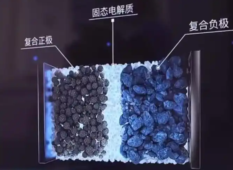
The broader context of my study is the need for safe, flexible, and mechanically robust energy storage in wearable electronics. Conventional lithium-ion batteries rely on liquid electrolytes, which introduce thermal runaway risks and mechanical rigidity. Those limitations are especially severe in wearable and textile-based applications. Solid electrolytes, particularly PEO-based systems, offer interfacial compatibility and tunable mechanical response. When a solid electrolyte is combined with fiber electrodes, the resulting all-solid-state fiber battery can be woven, stretched, and integrated into fabrics. The fiber electrode network provides efficient electron transport pathways and a large interfacial contact area. This geometry improves ion migration paths and enables rapid movement of ions between the electrode and the electrolyte. However, the same geometry also creates transport bottlenecks when the electrolyte layer is thick. My simulation work examines those bottlenecks quantitatively.
I organize the model around four coupled physical processes: solid-phase lithium diffusion inside active particles, ionic transport inside the solid electrolyte, electronic charge conservation inside the electrodes, and Butler-Volmer interfacial kinetics at the electrode/electrolyte boundaries. Each process is represented by a governing equation. The solid-phase diffusion equation is written as follows:
$$ \varepsilon \frac{\partial c_s}{\partial t} = \nabla \cdot \left( D_s \nabla c_s \right) + \frac{j_{\mathrm{int}}}{F} $$
Here, \(c_s\) is the lithium concentration in the solid active material, \(D_s\) is the solid-phase diffusion coefficient, \(\varepsilon\) is the volume fraction of the active material, \(j_{\mathrm{int}}\) is the interfacial reaction current density, and \(F\) is the Faraday constant. This equation captures how lithium enters and leaves the active particles during charge and discharge. In my solid state cell model, the active particles are treated as spherical particles with a uniform radius. I neglect phase transformation, gas generation, and dendrite growth in the baseline simulation. These assumptions keep the model tractable while preserving the dominant transport physics.
Inside the solid electrolyte, lithium ions move under the combined influence of diffusion and migration. I use a modified Nernst-Planck equation to describe this behavior:
$$ \frac{\partial c_{\mathrm{Li}^+}}{\partial t} = \nabla \cdot \left[ D_{\mathrm{eff}} \left( \nabla c_{\mathrm{Li}^+} + \frac{z F}{R T} c_{\mathrm{Li}^+} \nabla \phi_e \right) \right] $$
In this expression, \(c_{\mathrm{Li}^+}\) is the lithium-ion concentration in the electrolyte, \(D_{\mathrm{eff}}\) is the effective diffusivity of the electrolyte, \(z\) is the charge number of the lithium ion, \(R\) is the gas constant, \(T\) is the absolute temperature, and \(\phi_e\) is the electrolyte potential. Because the electrolyte is solid, there is no separate liquid-phase diffusion equation. Instead, the ionic transport equation for the solid electrolyte replaces the conventional liquid-phase treatment. This distinction is essential for a solid state cell, where ion conduction occurs through polymer chain segments or lattice sites rather than through a liquid solvent.
Charge conservation in the electrolyte and in the solid electrodes is expressed through the following equations:
$$ \nabla \cdot \left( k_{\mathrm{eff}} \nabla \phi_e \right) = – F \nabla \cdot \left( D_{\mathrm{eff}} \nabla c_{\mathrm{Li}^+} \right) $$
$$ \nabla \cdot \left( \sigma_e \nabla \phi_e \right) = – j_{\mathrm{int}} $$
$$ \nabla \cdot \left( \sigma_{\mathrm{eff}} \nabla \phi_s \right) = j_{\mathrm{int}} $$
Here, \(k_{\mathrm{eff}}\) is the effective ionic conductivity of the electrolyte, \(\sigma_e\) is the effective ionic conductivity used in the potential equation, \(\sigma_{\mathrm{eff}}\) is the effective electronic conductivity of the electrode, and \(\phi_s\) is the electrode potential. The first equation accounts for the coupling between ionic concentration gradients and electric potential in the solid electrolyte. The second equation describes how the interfacial current density drives ionic current in the electrolyte. The third equation describes electronic current in the solid electrode matrix. Together, these equations enforce charge conservation across the solid state cell.
The interfacial charge-transfer kinetics at the electrode/electrolyte interface are described by the Butler-Volmer equation:
$$ j = j_0 \left[ \exp \left( \frac{\alpha_a F \eta}{R T} \right) – \exp \left( – \frac{\alpha_c F \eta}{R T} \right) \right] $$
In this equation, \(j_0\) is the exchange current density, \(\alpha_a\) is the anodic transfer coefficient, \(\alpha_c\) is the cathodic transfer coefficient, and \(\eta\) is the overpotential. The overpotential is defined as the difference between the electrode potential and the electrolyte potential, shifted by the equilibrium potential:
$$ \eta = \phi_s – \phi_e – U_{\mathrm{eq}} $$
The exchange current density depends on the lithium concentration in the electrolyte and in the active material:
$$ j_0 = F k_0 c_{\mathrm{Li}^+}^{\alpha_a} \left( c_{\max} – c_s \right)^{\alpha_c} $$
Here, \(k_0\) is the reaction rate constant, \(c_{\max}\) is the maximum lithium concentration in the electrode, and \(c_s\) is the local lithium concentration in the solid active material. I also include a temperature-dependent rate constant:
$$ k_0 = k_{\mathrm{ref}} \exp \left[ \frac{E_a}{R} \left( \frac{1}{T_{\mathrm{ref}}} – \frac{1}{T} \right) \right] $$
In this expression, \(k_{\mathrm{ref}}\) is the reference reaction rate constant, \(E_a\) is the activation energy, \(T_{\mathrm{ref}}\) is the reference temperature, and \(T\) is the operating temperature. Although my baseline simulations are isothermal, this term allows the model to capture temperature-dependent interfacial kinetics when needed. In the solid state cell, the interface between the polymer electrolyte and the fiber electrode is a critical region. The Butler-Volmer formulation links the local potential difference to the local reaction rate, and therefore links electrolyte thickness to the overall electrochemical response.
To keep the model transparent, I summarize the main symbols and their physical meanings in the following table.
| Symbol | Meaning | Typical unit |
|---|---|---|
| \(c_s\) | Lithium concentration in solid active material | mol m\(^{-3}\) |
| \(c_{\mathrm{Li}^+}\) | Lithium-ion concentration in solid electrolyte | mol m\(^{-3}\) |
| \(D_s\) | Solid-phase diffusion coefficient | m\(^2\) s\(^{-1}\) |
| \(D_{\mathrm{eff}}\) | Effective electrolyte diffusivity | m\(^2\) s\(^{-1}\) |
| \(\phi_s\) | Electrode potential | V |
| \(\phi_e\) | Electrolyte potential | V |
| \(j_{\mathrm{int}}\) | Interfacial reaction current density | A m\(^{-2}\) |
| \(j_0\) | Exchange current density | A m\(^{-2}\) |
| \(\eta\) | Overpotential | V |
| \(\sigma_{\mathrm{eff}}\) | Effective electronic conductivity | S m\(^{-1}\) |
| \(\sigma_e\) | Effective ionic conductivity | S m\(^{-1}\) |
| \(\varepsilon\) | Active material volume fraction | dimensionless |
| \(F\) | Faraday constant | C mol\(^{-1}\) |
| \(R\) | Gas constant | J mol\(^{-1}\) K\(^{-1}\) |
| \(T\) | Temperature | K |
The model parameters I use for the LFP/LTO solid state cell are summarized below. These values define the baseline electrochemical and transport properties of the positive electrode, the negative electrode, and the solid electrolyte.
| Parameter | LFP positive electrode | LTO negative electrode | Solid electrolyte |
|---|---|---|---|
| Solid-phase potential (V) | 0.363 | 0.300 | Not applicable |
| Reference exchange current density (A m\(^{-2}\)) | 0.00304 | 0.00543 | Not applicable |
| Diffusion coefficient (m\(^2\) s\(^{-1}\)) | \(3.2 \times 10^{-13}\) | \(6.8 \times 10^{-15}\) | Not applicable |
| Electronic conductivity (S m\(^{-1}\)) | 91 | 100 | Not applicable |
| Equilibrium potential temperature derivative (V K\(^{-1}\)) | \(-9.95 \times 10^{-5}\) | \(-1.04 \times 10^{-5}\) | Not applicable |
| Maximum lithium concentration (mol m\(^{-3}\)) | 21190 | 22852 | Not applicable |
| Particle radius (m) | \(1 \times 10^{-9}\) | \(1 \times 10^{-9}\) | Not applicable |
| Ionic conductivity (S m\(^{-1}\)) | Not applicable | Not applicable | \(1.19 \times 10^{-2}\) |
I construct the geometry as a three-layer coaxial fiber structure. The inner core is a conductive stainless-steel strand. A LFP fiber electrode surrounds the core. A PEO-based solid electrolyte layer separates the LFP electrode from the outer LTO fiber electrode. The outer LTO layer is itself a fibrous network. This architecture makes the device a true fiber-shaped solid state cell. The electrolyte thickness is the key geometric variable in my study. I choose three nominal thicknesses: 30 \(\mu\)m, 45 \(\mu\)m, and 90 \(\mu\)m. I label these variants L30, L45, and L90. The fiber battery morphology was examined by scanning electron microscopy. The observations confirm that the fibers are orderly and that active material and conductive additive are uniformly distributed on the fiber surfaces. The electrolyte layer adheres closely to the LFP fiber electrode and forms a continuous intermediate layer. The outer LTO electrode layer appears as ordered nanofibers. The three layers are tightly integrated.
I use the finite element method to discretize the coupled equations over the three-dimensional fiber geometry. The model includes time-dependent diffusion, ionic migration, electronic conduction, and interfacial reaction kinetics. I apply no-flux boundary conditions at the outer boundaries, and I apply current or voltage control at the current collectors depending on the simulation step. The mesh is refined near the electrode/electrolyte interfaces because the reaction rate and the potential gradients are largest there. I verify mesh convergence by refining the interfacial mesh until the predicted voltage and current density change by less than a small tolerance. This procedure ensures that the numerical solution is not controlled by discretization error. The resulting model enables me to analyze the solid state cell at the microscopic scale.
Before using the model for thickness prediction, I validate it against experimental data. I compare the simulated voltage curve with the measured voltage curve for the LFP/LTO all-solid-state fiber battery. The two curves agree closely in three important features. First, the initial discharge voltage plateau is reproduced. Second, the gradual voltage decline during the middle of discharge is captured. Third, the sharp voltage drop near the end of discharge is predicted. This agreement indicates that the model accurately reflects the core electrochemical behavior of the solid state cell during discharge. The relationship between simulated and experimental specific capacity also corresponds well. Therefore, I conclude that the model is reasonable for describing capacity release and for predicting thickness-dependent performance trends.
| Discharge feature | Experimental observation | Simulated prediction | Agreement |
|---|---|---|---|
| Initial voltage plateau | Flat plateau near the beginning of discharge | Flat plateau reproduced | High |
| Middle-stage decline | Slow and gradual voltage decrease | Slow and gradual decrease | High |
| End-stage drop | Rapid voltage fall near end of discharge | Rapid fall reproduced | High |
| Specific capacity trend | Measured capacity release | Simulated capacity release | Reasonable |
After validation, I investigate the effect of electrolyte thickness on current density distribution. Current density in the electrolyte is a key indicator of electrochemical uniformity. It reflects how consistently ions are transported and how uniformly the electrode reactions proceed. When the solid state cell is discharged to 50% depth of discharge (DOD), the predicted current density distributions differ significantly among L30, L45, and L90. For L30, the current density distribution is relatively uniform. For L45, the current density gradient increases noticeably. For L90, the current density exhibits a pronounced layered gradient. This behavior is caused by the longer lithium-ion migration path in a thicker electrolyte. As thickness increases, lithium ions must travel a longer distance from the positive electrode to the negative electrode. During this journey, they must overcome more barriers, including polymer chain segmental resistance and local lattice or site-hopping resistance. The resistance per unit distance accumulates, so the electrolyte potential gradient along the thickness direction becomes steeper. Under discharge current, each unit length of the longer path contributes an additional potential loss. Therefore, the overall potential gradient becomes more pronounced as the electrolyte becomes thicker.
From the perspective of current density distribution, a thicker electrolyte increases the distance between regions where ions are consumed and regions where ions are replenished. Near the reaction front, lithium ions are consumed by the interfacial reaction. Near the opposite side, ions must be supplied by transport from the bulk. When the transport path is long, the replenishment at the far end cannot keep pace with consumption. This creates an ion transport lag. The lag produces a more significant concentration gradient inside the electrolyte. According to the Nernst equation, a local lithium-ion concentration difference translates directly into a local potential difference. In a thick electrolyte, the long path amplifies this concentration-to-potential conversion. Consequently, the spatial heterogeneity of the potential distribution is much greater in L90 than in L30. As discharge proceeds, continuous ion consumption and transport lag reinforce each other. Ohmic polarization and concentration polarization accumulate more strongly in the thick electrolyte. This is a central finding of my simulation study of the solid state cell.
I further analyze the time evolution of current density. When the solid state cell is discharged under a fixed demand, electrolyte thickness strongly regulates the dynamic current density. Over a discharge period from 0 s to 20,000 s, the maximum electrolyte current density is 0.207 A m\(^{-2}\) for L30, 0.214 A m\(^{-2}\) for L45, and 0.223 A m\(^{-2}\) for L90. These results show that increasing electrolyte thickness raises the internal current density. The reason is that the ion migration path is longer. To satisfy the same charge transfer rate, the system must increase the ionic flux per unit area, which is the current density, to compensate for the time delay caused by long-distance transport. The effect of thickness on current density is cumulative. It also intensifies the spatial and temporal non-uniformity of ion transport, which further amplifies polarization. In a solid state cell, this feedback is important because it can accelerate local degradation and reduce effective capacity.
| Electrolyte variant | Nominal thickness (\(\mu\)m) | Maximum current density over 20,000 s (A m\(^{-2}\)) | Observed distribution at 50% DOD |
|---|---|---|---|
| L30 | 30 | 0.207 | Relatively uniform |
| L45 | 45 | 0.214 | Increased gradient |
| L90 | 90 | 0.223 | Pronounced layered gradient |
The potential distribution in the electrolyte provides further evidence for the same mechanism. At 0% DOD, before significant discharge has occurred, the electrolyte potential difference is already different among the three variants. I obtain 0.6 mV for L30, 0.08 mV for L45, and 1.5 mV for L90. These values indicate that even in the un-discharged state, a thicker electrolyte can develop an initial potential gradient because of path-length differences. The physical origin is that when the electrolyte thickness increases, the lithium-ion migration path from the positive electrode to the negative electrode becomes longer. Ions must overcome more spatial transport resistance. Even at the beginning of discharge, the thicker electrolyte exhibits a more pronounced transport inertia difference. Ions near the positive electrode have not yet fully diffused to the negative side, while the ion concentration at the far end already differs because of the initial distribution. This path-length-induced polarization appears directly as an initial potential gradient. For the solid state cell, such initial gradients can influence the subsequent reaction distribution and can shift the local operating point of the electrode/electrolyte interface.
| Electrolyte variant | Thickness (\(\mu\)m) | Potential difference at 0% DOD (mV) | Implication |
|---|---|---|---|
| L30 | 30 | 0.6 | Smaller initial path-length polarization |
| L45 | 45 | 0.08 | Lowest measured initial difference in this set |
| L90 | 90 | 1.5 | Largest initial path-length polarization |
To interpret the thickness dependence more generally, I express the ionic resistance of the solid electrolyte layer in a simplified one-dimensional form. For a uniform electrolyte of thickness \(L\), cross-sectional area \(A\), and effective ionic conductivity \(\sigma_e\), the ionic resistance is:
$$ R_{\mathrm{ion}} = \frac{L}{\sigma_e A} $$
The ohmic potential drop across the electrolyte under a current \(I\) is therefore:
$$ \Delta \phi_{\mathrm{ohm}} = I R_{\mathrm{ion}} = \frac{I L}{\sigma_e A} $$
This simple relation already shows that increasing \(L\) increases the ohmic overpotential linearly when \(I\), \(\sigma_e\), and \(A\) are fixed. In a fiber-shaped solid state cell, the effective area and the current distribution are not perfectly one-dimensional, but the scaling remains informative. A thicker electrolyte increases the internal resistance. The increased resistance raises the ohmic overpotential. At the same time, the longer diffusion path increases the concentration overpotential. The concentration overpotential can be approximated through a Nernstian expression:
$$ \eta_{\mathrm{conc}} \approx \frac{R T}{F} \ln \left( \frac{c_{\mathrm{Li}^+,\mathrm{surface}}}{c_{\mathrm{Li}^+,\mathrm{bulk}}} \right) $$
Here, \(c_{\mathrm{Li}^+,\mathrm{surface}}\) is the lithium-ion concentration near the reaction interface and \(c_{\mathrm{Li}^+,\mathrm{bulk}}\) is the bulk concentration in the electrolyte. When the electrolyte is thick, the surface concentration deviates more strongly from the bulk value because ion replenishment is slower. Therefore, the logarithmic term grows, and the concentration overpotential increases. The total overpotential is approximately the sum of ohmic, concentration, and charge-transfer contributions:
$$ \eta_{\mathrm{total}} \approx \eta_{\mathrm{ohm}} + \eta_{\mathrm{conc}} + \eta_{\mathrm{ct}} $$
In my simulations, the charge-transfer contribution is governed by the Butler-Volmer equation. The ohmic and concentration contributions grow significantly with electrolyte thickness. This explains why the voltage plateau declines faster and why the end-of-discharge voltage is lower in the thicker solid state cell. The internal potential gradient becomes steeper, the internal resistance becomes larger, and both ohmic and concentration overpotentials increase. These effects reduce the usable capacity and can degrade rate performance.
I summarize the thickness-dependent trends in the following table. The table is intended to connect geometric variation to electrochemical consequences in a compact way.
| Increasing electrolyte thickness | Direct physical effect | Electrochemical consequence |
|---|---|---|
| Longer lithium-ion migration path | Higher cumulative transport resistance | Larger internal resistance |
| Longer diffusion distance | Stronger ion transport lag | Larger concentration gradient |
| Larger concentration gradient | Greater Nernstian potential difference | Larger concentration overpotential |
| Higher ionic resistance | Larger \(I R_{\mathrm{ion}}\) drop | Larger ohmic overpotential |
| Higher current density demand | Increased ionic flux per area | More non-uniform current distribution |
| Steeper potential gradient | More heterogeneous reaction rate | Faster voltage plateau decline |
| Slower ion replenishment | Lower surface concentration near interface | Lower end-of-discharge voltage |
The simulation results also reveal that the current density distribution and the potential distribution are tightly coupled. In a solid state cell, the electrolyte potential \(\phi_e\) and the lithium-ion concentration \(c_{\mathrm{Li}^+}\) are linked through the modified Nernst-Planck equation. When the electrolyte is thick, a small change in concentration can produce a larger change in potential because the transport path is long and the local concentration polarization is strong. This coupling modifies the local overpotential \(\eta = \phi_s – \phi_e – U_{\mathrm{eq}}\). As a result, the local reaction rate \(j\) changes according to the Butler-Volmer equation. Regions with higher overpotential react faster, while regions with lower overpotential react slower. This spatial variation in reaction rate further reinforces the current density gradient. The feedback loop is more severe in thicker electrolytes. Therefore, thickness is not merely a geometric parameter; it is an electrochemical design variable that controls the uniformity and efficiency of the solid state cell.
I also note that the fiber architecture introduces radial transport effects. Ions move not only along the fiber axis but also across the coaxial layers. The radial distance through the electrolyte is the thickness \(L\). The axial direction provides a long-range conduction path. When \(L\) is small, radial transport is fast, and the electrolyte can supply ions to the reaction interface efficiently. When \(L\) is large, radial transport becomes the limiting step. The reaction interface may become starved of ions even if the bulk electrolyte still contains sufficient lithium. This starvation increases the local overpotential and reduces the effective utilization of the active material. In my simulations, the L90 variant shows the strongest evidence of this behavior, especially near the end of discharge. The L30 variant maintains a more uniform reaction distribution because its radial transport length is shorter.
The validation against experimental voltage curves supports the use of the model as a predictive tool. The simulated curves reproduce the discharge plateau, the gradual decline, and the final drop. The capacity trend also aligns with measurements. This gives me confidence that the thickness-dependent trends I predict are physically meaningful. The model can therefore be used to screen electrolyte thicknesses before extensive experimental fabrication. It can also guide the design of fiber electrodes and the optimization of coating or spinning processes. In a solid state cell, reducing electrolyte thickness without causing short circuits or mechanical failure is a key pathway to higher power density and better rate capability. My results quantify the penalty associated with thicker electrolytes and show why thin, uniform, and continuous electrolyte layers are desirable.
The following table summarizes the three thickness variants and their predicted electrochemical behavior in a comparative format.
| Variant | Thickness (\(\mu\)m) | Current density uniformity | Potential gradient | Internal resistance | Ohmic overpotential | Concentration overpotential |
|---|---|---|---|---|---|---|
| L30 | 30 | High | Low | Lowest | Lowest | Lowest |
| L45 | 45 | Moderate | Moderate | Moderate | Moderate | Moderate |
| L90 | 90 | Low | High | Highest | Highest | Highest |
I also examine how the interfacial reaction kinetics respond to thickness. The exchange current density \(j_0\) depends on the local lithium concentration in the electrolyte and in the solid active material. In a thick electrolyte, the local electrolyte concentration near the reaction interface can deviate from the nominal value. This deviation changes \(j_0\). The Butler-Volmer current then changes, which alters the local consumption rate. The coupling between \(j_0\), \(c_{\mathrm{Li}^+}\), and \(\eta\) creates a nonlinear response. In my simulations, the nonlinearity is stronger for L90. This means that the solid state cell with a thick electrolyte is more sensitive to local transport limitations. It also means that simple linear extrapolation from thin to thick electrolytes may underestimate the performance loss. The finite element method captures this nonlinearity by solving the coupled equations simultaneously at each mesh point and each time step.
The temperature-dependent rate constant \(k_0\) is another important factor. If the solid state cell operates at a temperature different from the reference temperature, the interfacial kinetics change. A higher temperature increases \(k_0\), which can partially compensate for transport limitations. However, a higher temperature may also accelerate degradation. In my baseline study, I keep the temperature constant and focus on thickness. The model framework nevertheless includes the temperature dependence, so future work can explore thermal effects. For a solid state cell intended for wearable applications, temperature management is important because the device may experience body heat, environmental heat, and self-heating during fast charging or discharging.
The mechanical properties of the PEO-based electrolyte also matter. PEO-based solid electrolytes have tunable mechanical response and good interfacial affinity. These properties allow the electrolyte to maintain contact with the fiber electrodes during bending and stretching. However, a thicker electrolyte layer may be more susceptible to mechanical deformation and may increase the overall device stiffness. My simulation does not explicitly model mechanical deformation, but the electrochemical trends I find provide a strong reason to keep the electrolyte thin. A thin electrolyte reduces ionic resistance, shortens the diffusion path, and improves current density uniformity. It also reduces the volume and mass of the solid state cell, which is beneficial for wearable energy storage.
The fiber electrode structure adds another layer of complexity. The LFP and LTO layers are not flat films; they are fibrous networks. The active material is distributed on the fibers, and the electrolyte penetrates the network. This three-dimensional structure increases the interfacial area. A larger interfacial area can support a higher total current for a given current density. However, it also means that the local transport paths are tortuous. In my model, I represent the three-dimensional structure through effective transport parameters and a coaxial geometry. This approach captures the dominant radial transport limitation while retaining computational efficiency. The model predicts that the electrolyte thickness is a first-order factor controlling the uniformity of the solid state cell. The fiber network helps with electron transport and interfacial contact, but it cannot eliminate the ionic transport penalty of a thick electrolyte.
I can express the relationship between thickness and characteristic diffusion time in a simple form. The diffusion time across the electrolyte is approximately:
$$ \tau_{\mathrm{diff}} \approx \frac{L^2}{D_{\mathrm{eff}}} $$
This square dependence shows that doubling the thickness quadruples the characteristic diffusion time. For L30, L45, and L90, the nominal thickness ratios are 1, 1.5, and 3. The corresponding diffusion time ratios are 1, 2.25, and 9. This rapid increase explains why the L90 variant exhibits such a strong concentration gradient and such pronounced concentration overpotential. The ionic resistance, by contrast, scales linearly with thickness. The combination of linear resistance growth and quadratic diffusion time growth produces a strongly nonlinear electrochemical penalty. This is a key insight from my simulation analysis of the solid state cell.
| Variant | Thickness ratio | Ionic resistance ratio | Diffusion time ratio | Expected polarization trend |
|---|---|---|---|---|
| L30 | 1.0 | 1.0 | 1.0 | Baseline |
| L45 | 1.5 | 1.5 | 2.25 | Moderate increase |
| L90 | 3.0 | 3.0 | 9.0 | Strong increase |
The current density results can be further interpreted through the concept of ionic flux. The current density \(i\) is related to the ionic flux \(N_{\mathrm{Li}^+}\) by:
$$ i = F z N_{\mathrm{Li}^+} $$
To maintain a fixed total current, a thicker electrolyte must sustain a higher local ionic flux if the effective transport area is reduced by concentration polarization. In my simulations, the maximum current density increases from 0.207 to 0.223 A m\(^{-2}\) as thickness increases from 30 to 90 \(\mu\)m. This increase is not large in absolute terms, but it is significant because it reflects a redistribution of ionic flux. The local current density in some regions may be much higher than the average. Such local hot spots can accelerate degradation and reduce cycle life. Therefore, thickness optimization is also a durability strategy for the solid state cell.
The potential distribution results at 0% DOD show that the initial state is not necessarily uniform. Even before discharge, the thicker electrolyte can have a larger potential difference. This initial non-uniformity can affect the first charge or discharge cycle. It can also influence the formation of the solid electrolyte interphase or other interfacial layers. In a solid state cell, the interfacial contact quality is critical. If the initial potential distribution is non-uniform, the interfacial reaction may be uneven, leading to local stress and potential delamination. My model suggests that thinner electrolytes promote a more uniform initial potential distribution, which is beneficial for stable cycling.
I should note that the model assumes no side reactions, no volume changes, spherical active particles, no phase transformation, no gas generation, and no dendrite growth. These assumptions are standard for a baseline electrochemical model. They allow me to isolate the effect of electrolyte thickness. In a real solid state cell, these additional phenomena may interact with thickness. For example, dendrite growth may be more likely in thinner electrolytes if mechanical strength is insufficient. Side reactions may consume lithium and reduce capacity. Volume changes may alter interfacial contact. My model provides a clean baseline that can be extended to include these effects. The finite element framework is flexible enough to incorporate additional physics in future work.
The practical implications of my findings are clear. For LFP/LTO all-solid-state fiber batteries, electrolyte thickness should be minimized while maintaining mechanical integrity and preventing short circuits. A thinner electrolyte reduces ionic resistance, shortens the diffusion path, decreases ohmic and concentration overpotentials, improves current density uniformity, and supports a higher usable capacity. The simulation results show that the penalty for increasing thickness is significant, especially when thickness triples. The L90 variant exhibits the largest potential gradient, the highest internal resistance, and the strongest polarization. The L30 variant exhibits the most uniform behavior. Therefore, I recommend that design efforts focus on thin, continuous, and uniform PEO-based electrolyte layers. Process optimization for spinning, coating, and infiltration should aim to reduce thickness without creating defects.
I also recommend that future simulations couple the electrochemical model with a mechanical model. Such a coupled model could predict the trade-off between thickness, mechanical strength, and electrochemical performance. It could also predict how bending and stretching affect ion transport in the solid state cell. For wearable applications, mechanical flexibility is as important as electrochemical performance. A multi-physics approach would provide a more complete design tool. In addition, thermal coupling could be included to study self-heating during fast charging. The temperature-dependent rate constant and the temperature-dependent transport properties could then be used to predict thermal runaway risk or performance limitations.
The following table summarizes the main design recommendations that follow from my simulation study.
| Design factor | Recommended direction | Expected benefit |
|---|---|---|
| Electrolyte thickness | Keep as thin as mechanically possible | Lower ionic resistance and shorter diffusion path |
| Thickness uniformity | Ensure uniform coating along the fiber | More uniform current density and potential |
| Interfacial contact | Maintain intimate electrode/electrolyte contact | Lower charge-transfer resistance |
| Fiber electrode architecture | Optimize porosity and active material loading | Higher interfacial area and better electron transport |
| Operating temperature | Manage within a safe range | Balance kinetics and degradation |
| Mechanical design | Couple electrochemical and mechanical models | Ensure flexibility without sacrificing performance |
In conclusion, I have developed a finite element model of an LFP/LTO all-solid-state fiber battery using COMSOL. The model couples solid-phase diffusion, ionic transport in a PEO-based solid electrolyte, electronic conduction in the electrodes, and Butler-Volmer interfacial kinetics. I validated the model against experimental voltage curves and found good agreement in plateau behavior, middle-stage decline, end-stage drop, and capacity trend. I then used the model to study the effect of electrolyte thickness on the electrochemical performance of the solid state cell. The results show that increasing electrolyte thickness significantly increases the internal potential gradient and internal resistance. This leads to larger ohmic overpotential and larger concentration overpotential. The current density becomes less uniform, and the maximum current density increases because the system must compensate for longer transport paths. The initial potential difference at 0% DOD also increases for the thickest electrolyte. These effects combine to reduce the voltage plateau and lower the end-of-discharge voltage. The characteristic diffusion time scales with the square of thickness, while ionic resistance scales linearly, so the penalty for thick electrolytes is strongly nonlinear. My study demonstrates that finite element simulation is a fast and efficient tool for predicting the electrochemical performance of solid state cells and for guiding the design of all-solid-state fiber batteries. It provides a theoretical basis for optimizing electrolyte thickness, improving interfacial transport, and enhancing the energy density, cycling stability, and safety of flexible solid state cells.
For future work, I plan to extend the model to include mechanical deformation, thermal coupling, and interfacial degradation. I also plan to compare simulations with cycling data over longer periods. Such extensions will allow me to study how thickness affects not only initial performance but also long-term reliability. The solid state cell remains a promising platform for wearable energy storage, and my results show that geometric design, especially electrolyte thickness, must be carefully controlled to realize its full potential. I believe that combined simulation and experimental iteration will accelerate the development of high-performance all-solid-state fiber batteries. The solid state cell can then be woven into fabrics, integrated into garments, and used to power sensors, communication modules, and other wearable electronic devices without compromising comfort or safety.