
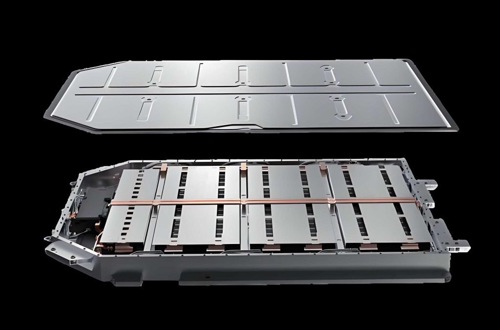
In my research, I focus on a critical quality-control problem in the manufacturing of high-performance electric vehicle battery packs: the automated detection of sealing nail welding defects. The sealing nail is a small but essential component of an electric vehicle battery pack because it isolates the electrolyte from the external environment after the injection process. When the sealing nail weld contains a burst, a missed weld, a pinhole, or a misaligned weld, the electric vehicle battery pack can suffer electrolyte leakage, thermal instability, and safety risks. My work therefore aims to build a robust, accurate, and automated point-cloud-based defect detection pipeline that can be deployed in an industrial environment.
1. Motivation and Problem Context
The rapid growth of new energy vehicles has placed increasing pressure on the production quality of electric vehicle battery packs. A modern electric vehicle battery pack accounts for a large fraction of vehicle cost, and its reliability directly influences driving range, service life, and occupant safety. Sealing nail welding is one of the final sealing steps in battery cell manufacturing. After electrolyte injection, the sealing nail must be welded onto the injection hole so that the electric vehicle battery pack is completely sealed. Contamination on the welding nozzle, fluctuations in laser power, and residual dirt in the welding area can introduce defects such as bursts, pits, molten beads, warpage, and pinholes.
Traditional inspection methods for sealing nail defects often rely on manual visual inspection or conventional two-dimensional image algorithms. Although two-dimensional imaging is fast and inexpensive, it struggles to represent depth, curvature, and three-dimensional geometry. For an electric vehicle battery pack, these geometric features are especially important because small changes in height or shape may indicate severe sealing failure. Manual inspection is also inefficient, subjective, and difficult to sustain over long production cycles. Consequently, I pursued a three-dimensional point-cloud approach that can capture the true surface morphology of the sealing nail and its welding region.
Conventional three-dimensional point-cloud algorithms can sometimes detect large geometric deviations, but they often fail when the defect is small, irregular, or embedded in a complex metallic surface. In my research, I observed that the sealing nail area contains strong noise from laser reflection, uneven surface roughness, and scanning artifacts. The defect regions are often extremely small relative to the full electric vehicle battery pack component, which creates a severe class imbalance. These issues motivate my use of deep learning on point clouds, especially graph-based semantic segmentation, to detect and segment sealing nail defects at the point level.
2. Research Objectives and Contributions
My overall objective is to improve the accuracy, robustness, and automation level of sealing nail defect detection for the electric vehicle battery pack production line. I divide the problem into four parts: point-cloud preprocessing, welding region extraction, defect semantic segmentation, and small-defect enhancement. Each part is designed to solve a specific failure mode observed in real industrial data. The main contributions of my work are summarized in the following table.
| Contribution | Problem Addressed | Method | Key Result |
|---|---|---|---|
| Improved point-cloud segmentation | Interference from the battery top cover and substrate in the electric vehicle battery pack point cloud | Improved random sample consensus with local sampling and misclassification correction | F1 score reached 87.74% |
| Improved graph attention network | Missed defect regions and weak local geometric feature extraction | Local graph attention filter and spatial attention graph pooling | mIoU and mAcc improved by 8.38% and 4.72% |
| Cross-density feature fusion | Low segmentation accuracy for small defects such as bursts, molten beads, and pinholes | Cross-attention-based cross-density feature fusion module | Small-defect IoU improved by 1.89%, 4.66%, and 5.08% |
| Automated inspection software | Lack of user-friendly visualization for non-specialists | GUI-based detection platform with model loading, welding region fitting, defect detection, and result saving | Automated detection and report generation |
These contributions are connected by a common theme: I aim to make point-cloud deep learning practical for the electric vehicle battery pack industry. Instead of treating the sealing nail as a generic object, I explicitly model the spatial relationship between the sealing nail, the welding region, and the surrounding top cover. This allows the detector to focus on the defect-prone area and ignore irrelevant background points.
3. Data Acquisition and Preprocessing
3.1 Point Cloud Acquisition
I used a line laser scanner to acquire the three-dimensional point cloud of the sealing nail on an electric vehicle battery pack. The scanner emits a laser line and captures the reflected profile, producing point coordinates with micrometer-level precision. The working distance, measurement range, and Z-axis resolution are suitable for small sealing nail features. During acquisition, the scanner moves across the sealing nail surface and collects the global point cloud, which contains only XYZ coordinates and does not include normal vectors, color, or curvature.
Because the raw data are obtained from a reflective metallic surface, the point cloud contains noise and outliers. These artifacts come from several sources: unstable laser reflection on rough welding areas, multiple reflections on the sealing nail surface, system errors from the scanner itself, and environmental disturbances such as dust or vibration. If I directly feed the raw electric vehicle battery pack point cloud into a deep network, the noise will reduce detection accuracy and increase computational cost. Therefore, I designed a preprocessing pipeline consisting of statistical filtering and welding region extraction.
3.2 Statistical Filtering Denoising
For denoising, I applied a statistical outlier removal filter. For each point \(p_i\), I compute the average distance to its \(k\) nearest neighbors:
$$
\tilde{d}_i = \frac{1}{k} \sum_{j=1}^{k} \sqrt{(x_i – x_{ij})^2 + (y_i – y_{ij})^2 + (z_i – z_{ij})^2}.
$$
I assume that the average distance follows a normal distribution \(N(\mu, \sigma^2)\). The mean and standard deviation are estimated as follows:
$$
\mu = \frac{1}{n} \sum_{i=1}^{n} \tilde{d}_i,
$$
$$
\sigma = \sqrt{\frac{1}{n} \sum_{i=1}^{n} (\tilde{d}_i – \mu)^2}.
$$
I set a distance threshold \(\varepsilon = \mu + \theta \sigma\). If a point has an average distance larger than \(\varepsilon\), it is treated as an outlier and removed. This operation significantly improves the signal-to-noise ratio of the electric vehicle battery pack sealing nail point cloud and provides a cleaner input for subsequent segmentation.
3.3 Improved Random Sample Consensus for Welding Region Extraction
The electric vehicle battery pack top cover and substrate occupy a large portion of the raw point cloud. If these points are not removed, the defect detector may confuse background geometry with true defects. I therefore developed an improved random sample consensus algorithm to extract the sealing nail and welding region. The original random sample consensus method randomly selects three points to fit a plane, counts inliers, and repeats the process. However, random sampling is inefficient for dense industrial point clouds and may fit false planes.
My improved method uses a local sampling strategy. First, I build a k-d tree and estimate the normal vector of each point. For a point \(p_i\), the covariance matrix \(C\) of its neighborhood is
$$
C = \frac{1}{n} \sum_{i=1}^{n} (p_i – \bar{p})(p_i – \bar{p})^T.
$$
The normal vector is the eigenvector corresponding to the smallest eigenvalue of \(C\). For a candidate seed point, I search its neighborhood within radius \(r\). If the average cosine similarity between the local normals and the vertical direction \(n_v = (0,0,1)\) is larger than a threshold, the neighborhood is considered likely to belong to the sealing nail or top cover plane. The average cosine value is
$$
\gamma = \frac{1}{n} \sum_{i=1}^{n} n_v \cdot n_i.
$$
I then randomly select three points from this local neighborhood as the minimal sample set. This local sampling strategy reduces the probability of fitting a spurious plane and accelerates convergence. After fitting multiple planes, I perform misclassification correction. For each point in a candidate plane cluster, I compute the perpendicular distance to the plane and the distance to the cluster centroid. If both distances are below thresholds, the point is considered a misclassified point. I then use a k-d tree to find its nearest neighbors and reassign it to the cluster with the largest number of neighboring points.
To handle over-segmentation, I apply Euclidean clustering. The Euclidean clustering algorithm groups points whose mutual distances are below a given threshold \(\delta\). After clustering, the sealing nail patch and the top cover patch are separated. The patch with fewer points is identified as the sealing nail, and the region at a radius of approximately 5–6.5 mm around the sealing nail centroid is defined as the welding region. The comparison of segmentation algorithms is shown in the following table.
| Segmentation Algorithm | Computation Time (s) | Precision (%) | Recall (%) | F1 Score (%) |
|---|---|---|---|---|
| Traditional RANSAC | 6.82 | 76.24 | 82.19 | 79.10 |
| Region Growing | 8.73 | 83.10 | 81.57 | 82.33 |
| Euclidean Clustering | 3.45 | 36.23 | 99.73 | 53.15 |
| My Improved Method | 6.14 | 82.44 | 93.76 | 87.74 |
The improved method achieves the highest F1 score and maintains a reasonable computation time. This is important for an electric vehicle battery pack production line, where both accuracy and cycle time matter. By extracting only the sealing nail and welding region, I reduce the point count and allow the deep network to focus on defect-prone geometry.
4. Deep Learning-Based Defect Detection
4.1 Baseline Graph Attention Network
For the defect detection backbone, I selected a graph attention convolution network. This network constructs a directed graph from the point cloud and applies attention-based convolution to local neighborhoods. The graph is defined as \(\mathcal{G} = (\mathcal{V}, \mathcal{E})\), where \(\mathcal{V}\) is the set of vertices and \(\mathcal{E}\) is the set of edges. For each point \(i\), its neighborhood is \(\mathcal{N}(i)\). The attention weight between vertex \(i\) and neighbor \(j\) is computed from both spatial and feature differences:
$$
e_{ij} = M_\alpha([\Delta p_{ij} \,\|\, \Delta h_{ij}]), \quad j \in \mathcal{N}(i),
$$
where \(\Delta p_{ij} = p_i – p_j\) and \(\Delta h_{ij} = M_g(h_i) – M_g(h_j)\). The weights are normalized using a softmax function:
$$
a_{ij} = \frac{\exp(e_{ij})}{\sum_{l \in \mathcal{N}(i)} \exp(e_{il})}.
$$
The output feature of vertex \(i\) is then
$$
h_i’ = \sum_{j \in \mathcal{N}(i)} a_{ij} \odot M_g(h_j) + b_i.
$$
Although this baseline is effective, I found two limitations in the sealing nail task. First, concatenating spatial and feature differences can mix coordinate information with semantic feature information. Second, the pooling operation may not fully preserve local geometric details, which is problematic for small defects on an electric vehicle battery pack sealing nail.
4.2 Local Graph Attention Filter
To address these limitations, I proposed a local graph attention filter module. Instead of directly concatenating spatial and feature differences, I model the correlation matrix using a subtraction operation:
$$
C_{ij} = \phi_q(x_i) – \phi_k(x_i – x_j), \quad i,j \in \mathcal{V}.
$$
Here, \(\phi_q\) and \(\phi_k\) are learnable linear functions that project features into a metric space. I also introduce a distance-based constraint on the adjacency matrix:
$$
\hat{A}_{ij} = A_{ij} \cdot e^{-\|p_i – p_j\|^2},
$$
$$
A’ = D^{-1/2} \hat{A} D^{-1/2}.
$$
The learnable spatial term is
$$
\sigma_{ij} = M_p(p_i – p_j),
$$
and the attention weight becomes
$$
e_{ij} = M_e(C_{ij} \cdot A’_{ij}).
$$
After softmax normalization, the final output is
$$
y_i = \psi(x_i) + \sum_{j \in \mathcal{N}(i)} a_{ij} \odot (\phi_v(x_i – x_j) + \sigma_{ij}).
$$
This module filters irrelevant long-range information while emphasizing local geometric details. In my experiments, this change improved the network’s ability to distinguish defect boundaries from normal sealing nail surface points.
4.3 Spatial Attention Graph Pooling
I further proposed a spatial attention graph pooling module to replace the standard graph pooling operation. The weight between vertex \(i\) and neighbor \(j\) is computed from spatial coordinates:
$$
\hat{r}_{ij} = M_w(\varphi_q(p_i) – \varphi_k(p_j)).
$$
After normalization,
$$
r_{ij} = \frac{\exp(\hat{r}_{ij})}{\sum_{l \in \mathcal{N}(i)} \exp(\hat{r}_{il})}.
$$
The pooled feature is
$$
F_i = \sum_{j \in \mathcal{N}(i)} r_{ij} \odot \varphi_v(F_{ij}).
$$
At each downsampling stage, I first perform farthest point sampling to reduce the point count. For example, from one pyramid level to the next, the number of points is reduced to one quarter. Then, for each sampled point, I apply spatial attention pooling on the original graph to aggregate features. This design allows the network to retain spatial context while reducing resolution, which is especially useful for small defect regions in an electric vehicle battery pack sealing nail.
4.4 Loss Function Optimization
Sealing nail defect detection is a multi-class semantic segmentation problem with severe class imbalance. Normal background points dominate the dataset, while defect points are rare. If I use a standard cross-entropy loss, the network may ignore small defects. I therefore assign class weights to the loss function. The weight for class \(i\) is
$$
w_i = \frac{\hat{w}_i}{\sum_{i=1}^{k} \hat{w}_i},
$$
where
$$
\hat{w} = \left[ \left(\frac{n_{\max}}{n_1}\right)^{1/2}, \left(\frac{n_{\max}}{n_2}\right)^{1/2}, \dots, \left(\frac{n_{\max}}{n_k}\right)^{1/2} \right].
$$
The weighted loss is
$$
Loss = – \sum_{i=1}^{k} w_i y_i \log \frac{\exp(x_i)}{\sum_{l=1}^{k} \exp(x_l)}.
$$
This optimization reduces the bias toward the background class and improves the recall of small defect regions. In my experiments, it helped the network detect pinholes and molten beads that would otherwise be missed.
5. Cross-Density Feature Fusion for Small Defects
Although the improved graph attention network performed well on large defects, I observed that small defects such as bursts, molten beads, and pinholes still suffered from low segmentation accuracy. These defects occupy only a few points in the electric vehicle battery pack sealing nail point cloud. The graph pyramid gradually reduces point density, which can erase fine geometric details. To solve this, I designed a cross-density feature fusion module based on cross-attention. The module fuses features from different pyramid levels so that deep semantic features can be combined with shallow high-density geometric features.
5.1 Overall Network Structure
The improved network, which I call LGANet-CDF, contains five pyramid levels. Information flows in three directions: horizontally within each level, downward from high-density to low-density levels, and upward from low-density to high-density levels. The horizontal flow preserves point density and integrates local information. The downward flow brings high-density detail into deeper levels. The upward flow brings deep semantic context into shallower levels. The fusion module combines these three types of information. The first level uses a simple skip connection, while the second level and above use the cross-density fusion module.
5.2 Feature Downsampling and Upsampling
For downward flow, I use a feature downsampling module to match the point count of the next level. Farthest point sampling reduces the number of points to one quarter. Then, for each sampled point, I perform graph pooling on the original graph. This produces a coarse feature map that aligns with the lower-density level. For upward flow, I use a feature upsampling module. Given the coordinates \(P_l\) and \(P_{l-1}\) and features \(X_l\), I find the \(k\) nearest neighbors of each point in \(P_{l-1}\) within \(P_l\). The interpolated feature is
$$
x_{l-1,i} = \frac{1}{norm} \sum_{j \in \mathcal{P}(i)} \frac{x_{l,j}}{\|p_{l-1,i} – p_{l,j}\|^2},
$$
$$
norm = \sum_{j \in \mathcal{P}(i)} \frac{1}{\|p_{l-1,i} – p_{l,j}\|^2}.
$$
This allows the network to restore fine spatial resolution for small defect segmentation.
5.3 Cross-Attention Fusion Module
The cross-density feature fusion module uses the middle-level feature as a query sequence. The lower-density and higher-density levels provide key and value sequences. For the shallow high-density branch, the output is
$$
y_{l-1,i} = \sum_{j \in \mathcal{N}_{l-1}(i)} \rho(\chi_q(x_l) \cdot \chi_k^{l-1}(x_{l-1})) \cdot \chi_v^{l-1}(x_{l-1}).
$$
For the deep low-density branch, the output is
$$
y_{l+1,i} = \sum_{j \in \mathcal{N}_{l+1}(i)} \rho(M(\chi_q(x_l) – \chi_k^{l+1}(x_{l+1}))) \odot \chi_v^{l+1}(x_{l+1}).
$$
Here, \(\chi_q\), \(\chi_k\), and \(\chi_v\) are linear functions, \(\rho\) is a softmax function, and \(M\) is a multilayer perceptron. The module then stacks the enhanced features and applies a multilayer perceptron to reduce dimensionality. The shallow branch emphasizes detail and boundary information, while the deep branch emphasizes semantic context. By combining them, the network can recognize small defects without losing global consistency.
6. Experiments and Results
6.1 Dataset and Augmentation
I collected point cloud samples from an electric vehicle battery pack sealing nail inspection station. The dataset includes normal samples and five defect categories: burst, pit, molten bead, warpage, and pinhole. The point count distribution is highly imbalanced. The following table summarizes the point counts in a subset of 600 samples.
| Category | Background | Burst | Pit | Molten Bead | Warpage | Pinhole |
|---|---|---|---|---|---|---|
| Point Count | 62,931,445 | 93,601 | 165,430 | 48,789 | 1,793,618 | 64,363 |
Most defect samples contain fewer than 1,000 defect points, except for warpage, which covers a larger area. This imbalance makes the detection of small defects challenging. To improve generalization, I applied affine transformations including rotation, translation, flipping, and scaling. I also used random jitter and random normal-vector dropout during training. The final dataset contains 2,787 samples. I split the data into training, validation, and test sets at a ratio of 9:1:1. The category distribution after augmentation is shown below.
| Category | Normal | Burst | Pit | Molten Bead | Warpage | Pinhole |
|---|---|---|---|---|---|---|
| Number of Samples | 655 | 406 | 271 | 248 | 316 | 361 |
6.2 Training Setup and Metrics
I trained the network on a GPU-accelerated workstation with a deep learning framework. The training parameters are listed in the following table.
| Parameter | Configuration |
|---|---|
| Epoch | 300 |
| Batch Size | 8 |
| Point Count per Sample | 16,384 |
| Optimizer | AdamW |
| Initial Learning Rate | 0.01 |
| Learning Rate Schedule | Multi-step decay |
I used four evaluation metrics: overall accuracy, mean class accuracy, class intersection over union, and mean intersection over union. Their definitions are
$$
OA = \frac{\sum_{i=1}^{k} n_{ii}}{\sum_{i=1}^{k} \sum_{j=1}^{k} n_{ij}},
$$
$$
mAcc = \frac{1}{k} \sum_{i=1}^{k} \frac{n_{ii}}{\sum_{j=1}^{k} n_{ij}},
$$
$$
IoU_i = \frac{P_{i,pred} \cap P_{i,true}}{P_{i,pred} \cup P_{i,true}},
$$
$$
mIoU = \frac{1}{k} \sum_{i=1}^{k} \frac{n_{ii}}{\sum_{j=1}^{k} n_{ij} + \sum_{j=1}^{k} (n_{ji} – n_{ii})}.
$$
Overall accuracy reflects the point-level correctness, while mean class accuracy balances the influence of rare classes. Mean intersection over union is especially important for small defects because it measures the overlap between the predicted defect region and the true defect region.
6.3 Comparison with Other Networks
I compared my improved network with several representative point-cloud semantic segmentation networks. The results on the sealing nail dataset are shown in the following table. My method achieved the highest overall accuracy, mean class accuracy, and mean intersection over union.
| Model | OA (%) | mAcc (%) | mIoU (%) | Burst IoU (%) | Pit IoU (%) | Molten Bead IoU (%) | Warpage IoU (%) | Pinhole IoU (%) |
|---|---|---|---|---|---|---|---|---|
| LGANet+CDF | 99.13 | 96.20 | 81.25 | 80.06 | 71.91 | 75.99 | 89.89 | 70.03 |
| GACNet | 96.68 | 87.96 | 70.85 | 56.88 | 67.52 | 54.64 | 87.93 | 59.37 |
| PointNet | 82.66 | 72.46 | 45.74 | 28.33 | 30.01 | 21.53 | 62.64 | 34.95 |
| PointNet++ | 89.33 | 84.65 | 62.67 | 47.91 | 59.32 | 42.37 | 81.64 | 46.53 |
| Point Transformer v1 | 98.77 | 90.96 | 72.83 | 68.54 | 62.83 | 58.37 | 89.67 | 58.37 |
| Point Transformer v3 | 99.03 | 94.96 | 75.13 | 77.32 | 67.98 | 60.44 | 89.17 | 56.21 |
| OA-CNN | 98.72 | 91.13 | 74.04 | 64.89 | 66.91 | 64.87 | 88.37 | 60.04 |
Compared with the baseline GACNet, my method improved OA by 2.45%, mAcc by 8.24%, and mIoU by 10.4%. The largest improvements were observed for burst and molten bead defects, which are small and irregular. This confirms that the cross-density feature fusion module is effective for small defect detection in an electric vehicle battery pack sealing nail.
To evaluate generalization, I also tested my network on a public sewer semantic segmentation dataset. The results are shown below. My method achieved the highest OA, mean F1-score, and mIoU among the compared networks.
| Model | OA (%) | mF1-score (%) | mIoU (%) | Spalling | Blockage | Corrosion | Misalign | Deposit | Displace | Rubber Ring |
|---|---|---|---|---|---|---|---|---|---|---|
| LGANet | 98.94 | 95.33 | 91.12 | 86.84 | 95.74 | 80.38 | 93.84 | 91.33 | 95.68 | 86.32 |
| DLNet | 97.51 | 87.26 | 79.24 | 64.51 | 94.90 | 42.28 | 87.88 | 77.82 | 89.18 | 79.84 |
| PointNeXt | 96.25 | 73.55 | 65.64 | 2.02 | 95.28 | 29.17 | 80.07 | 68.40 | 85.07 | 68.83 |
| DeepGCN | 83.96 | 41.73 | 32.68 | 3.58 | 59.64 | 1.82 | 9.65 | 40.09 | 30.18 | 31.54 |
| DGCNN | 82.96 | 44.36 | 28.29 | 1.06 | 51.36 | 8.99 | 5.63 | 16.75 | 23.17 | 34.85 |
| PointNet++ | 83.42 | 42.31 | 32.22 | 0.00 | 30.27 | 17.32 | 25.55 | 66.94 | 18.53 | 8.07 |
6.4 Ablation Studies
I performed ablation studies to evaluate the contribution of each proposed module. The first ablation study examines the local graph attention filter and spatial attention graph pooling. The results are shown below.
| LGAF | SAG Pooling | OA (%) | mAcc (%) | mIoU (%) |
|---|---|---|---|---|
| No | No | 96.68 | 87.96 | 70.85 |
| Yes | No | 97.38 | 90.14 | 77.17 |
| No | Yes | 97.96 | 88.95 | 74.81 |
| Yes | Yes | 99.47 | 92.68 | 79.23 |
Both modules improve the baseline, and their combination yields the best performance. The mAcc improvement of 4.72% indicates fewer missed and false defect points. The mIoU improvement of 8.38% indicates better boundary segmentation of defect regions.
The second ablation study examines the information flow in the cross-density fusion module. The results are shown below.
| Down-flow | Up-flow | Burst IoU (%) | Pit IoU (%) | Molten Bead IoU (%) | Warpage IoU (%) | Pinhole IoU (%) |
|---|---|---|---|---|---|---|
| No | No | 78.17 | 72.17 | 71.33 | 91.61 | 64.95 |
| Yes | No | 79.63 | 71.24 | 74.31 | 87.64 | 71.37 |
| No | Yes | 76.62 | 73.81 | 71.12 | 92.94 | 63.14 |
| Yes | Yes | 80.06 | 71.91 | 75.99 | 89.89 | 70.03 |
The downward flow improves small defect detection by preserving high-density geometric details. The upward flow improves large defect detection by providing semantic context. Using both flows provides a balanced improvement across all defect categories.
The third ablation study evaluates where to insert the cross-density fusion module. The results are shown below.
| Configuration | mAcc (%) | mIoU (%) | ΔmIoU (%) |
|---|---|---|---|
| Baseline LGANet | 92.68 | 79.23 | — |
| Fusion at one low level | 92.32 | 78.96 | -0.27 |
| Fusion at one middle level | 94.03 | 80.11 | +0.88 |
| Fusion at two middle levels | 96.20 | 81.25 | +2.02 |
| Fusion at three levels | 94.97 | 80.69 | +1.46 |
The best configuration uses fusion at two middle levels. This provides a balance between high-resolution detail and deep semantic context. Adding fusion at too many levels increases computational complexity and may introduce redundant information.
6.5 Robustness to Point Density
I also tested the robustness of my model under different point densities. I randomly sampled 16,384, 8,192, 4,096, and 2,048 points from each test sample. The accuracy of my model decreased by less than 2% when the point count was reduced from 16,384 to 4,096. In contrast, other networks showed larger performance drops. This indicates that my network is robust to sparse point clouds, which is important for industrial electric vehicle battery pack inspection where scanning conditions may vary.
7. Software Platform for Automated Inspection
To make the proposed method usable by non-specialists, I developed a software platform for sealing nail defect detection. The platform provides a graphical user interface that allows a user to load a trained model, select a point cloud sample, fit the welding region, run detection, and save the results. The interface displays both the original depth map and the detection result. The system supports five defect types: burst, pit, molten bead, warpage, and pinhole.
The workflow of the software platform is as follows. First, the user selects a pretrained weight file. Second, the user selects a point cloud sample, and the system converts it into a depth image. Third, the user enters the inner and outer radii of the welding ring according to the sealing nail dimensions. Fourth, the system fits the welding region and highlights it. Fifth, the user clicks the detection button, and the system classifies the defect points. If a defect is found, the defect region is marked in the visualization. Finally, the user can save the defect data as a text file, including defect type, defect count, and remarks.
This software platform is designed to support automated quality control in electric vehicle battery pack manufacturing. It reduces the reliance on expert operators and provides a repeatable, data-driven inspection process. The platform can be integrated into a production line where each electric vehicle battery pack sealing nail is scanned and evaluated automatically.
8. Conclusions and Future Work
In my research, I developed a point-cloud deep learning method for sealing nail defect detection in an electric vehicle battery pack. The method includes an improved random sample consensus algorithm for welding region extraction, a local graph attention filter, a spatial attention graph pooling module, and a cross-density feature fusion module. Experimental results show that the proposed method significantly improves defect detection accuracy and small-defect segmentation performance. The F1 score of welding region extraction reached 87.74%. The improved network increased mIoU and mAcc by 8.38% and 4.72% over the baseline. The cross-density fusion module further improved the IoU of burst, molten bead, and pinhole defects by 1.89%, 4.66%, and 5.08%, respectively. Compared with the original baseline, the final model improved mIoU and mAcc by 10.4% and 8.24%.
Despite these results, there are several directions for future work. First, I plan to expand the dataset with more diverse electric vehicle battery pack samples, including different materials, surface finishes, and lighting conditions. This will improve generalization across production lines. Second, I will explore lightweight network architectures and hardware acceleration to reduce inference time for real-time inspection. Third, I will investigate multimodal fusion of three-dimensional point clouds and two-dimensional grayscale images to combine geometric and texture information. Fourth, I will study online learning and adaptive updating so that the model can adapt to new defect patterns without frequent manual retraining.
Overall, my work provides a practical and accurate approach for sealing nail defect detection in electric vehicle battery pack manufacturing. By combining improved point-cloud preprocessing, graph attention learning, cross-density feature fusion, and a user-friendly software platform, I aim to support higher automation levels, better quality control, and safer electric vehicle battery pack production.