
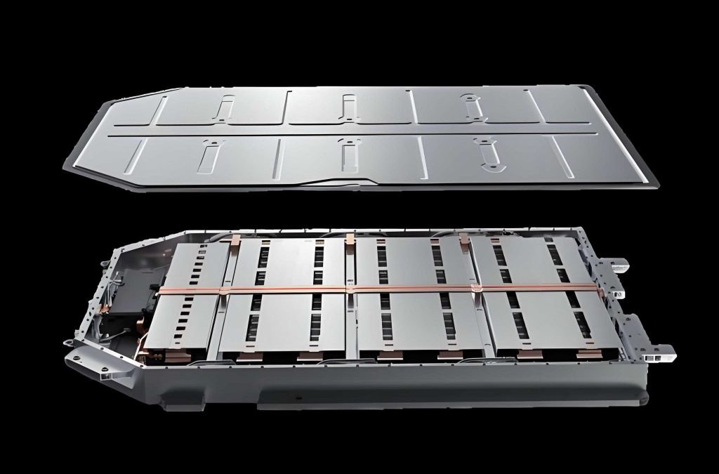
In my work, I treat the electric vehicle battery pack as a coupled thermal, hydraulic, and structural system. The electric vehicle battery pack must deliver the required energy and power while keeping every cell within a safe temperature window, and it must also protect the cells against road-induced mechanical loads. I therefore developed a complete design workflow in which I first estimate the pack energy and power requirements, then design the cell arrangement, then create and optimize a liquid-cooling thermal management system, and finally verify and improve the enclosure structure. The main design target is an electric vehicle battery pack with a usable energy of approximately 40.5 kWh, a maximum discharge rate of 3C, a liquid-cooling plate based on a 50 wt% ethylene glycol solution, and an aluminum enclosure that remains safe under severe acceleration and random vibration. I use computational fluid dynamics and finite element analysis as the main numerical tools, and I combine parametric studies, response surface approximations, and a non-dominated sorting genetic algorithm for multi-objective improvement.
Thermal Characteristics of Lithium-Ion Cells
I begin with the heat generation mechanism because the entire thermal management design depends on how much heat the cells produce and how that heat can be removed. A lithium-ion cell stores and releases energy through the migration of lithium ions between the positive and negative electrodes. During discharge, lithium ions move from the negative electrode to the positive electrode, and electrons flow through the external circuit. The main reversible and irreversible heat sources are electrochemical reaction heat, polarization heat, ohmic heat, and side-reaction heat. Under normal operation, side reactions are small and can be neglected. The total heat generation rate used in my models is represented by
$$Q = I^2 R + I T \frac{dU_{ocv}}{dT}$$
where \(Q\) is the total heat generation rate, \(I\) is the discharge current, \(R\) is the internal resistance, \(T\) is the cell temperature, and \(U_{ocv}\) is the open-circuit voltage. This form shows that internal resistance is a dominant contributor to temperature rise. I therefore treat the cell as a volumetric heat source with equivalent thermal properties, and I use the Bernardi-type heat generation rate to define the source term in the electric vehicle battery pack simulations.
Heat transfer inside and around the electric vehicle battery pack occurs mainly by conduction and convection. Radiation is present but is small in the temperature range of interest, so I neglect it. Fourier’s law for conduction is
$$\Phi = -\lambda A \frac{dt}{dx}$$
where \(\Phi\) is the heat flow, \(\lambda\) is the thermal conductivity, \(A\) is the cross-sectional area, and \(dt/dx\) is the temperature gradient. Convection follows Newton’s law of cooling:
$$\Phi = h A (t_w – t_f)$$
where \(h\) is the convective heat transfer coefficient, \(t_w\) is the wall temperature, and \(t_f\) is the fluid temperature. For internal flow in the cooling plate, the Nusselt number is
$$Nu = \frac{h d}{\lambda_l}$$
and the Gnielinski correlation gives a high-accuracy estimate for turbulent flow:
$$Nu = \frac{(f/8)(Re-1000)Pr}{1+12.7\sqrt{f/8}(Pr^{2/3}-1)}\left[1+\left(\frac{d}{l}\right)^{2/3}\right]$$
where \(f\) is the Darcy friction factor, \(Re\) is the Reynolds number, \(Pr\) is the Prandtl number, \(d\) is the hydraulic diameter, and \(l\) is the channel length. The friction factor is
$$f = (1.8 \log Re – 1.5)^{-2}$$
and the Reynolds number is
$$Re = \frac{\rho u d}{\mu}$$
where \(\rho\) is density, \(u\) is velocity, and \(\mu\) is dynamic viscosity. Flow resistance is divided into major and minor losses:
$$\Delta P_\lambda = \lambda \frac{l}{d}\frac{\rho v^2}{2}$$
$$\Delta P_r = \zeta \frac{\rho v^2}{2}$$
where \(\lambda\) is the major loss coefficient, \(\zeta\) is the minor loss coefficient, \(l\) is the channel length, \(d\) is the hydraulic diameter, \(\rho\) is fluid density, and \(v\) is fluid velocity. These equations explain why a well-designed electric vehicle battery pack cooling plate should increase contact area and reduce unnecessary vortex formation rather than simply increase flow rate.
For the fluid domain, I solve the mass, momentum, and energy conservation equations. For an incompressible coolant, they are
$$\nabla \cdot \mathbf{v} = 0$$
$$\rho\left(\frac{\partial \mathbf{v}}{\partial t}+\mathbf{v}\cdot\nabla\mathbf{v}\right)=-\nabla P+\mu\nabla^2\mathbf{v}+\rho\mathbf{g}$$
$$\rho c_p\left(\frac{\partial T}{\partial t}+\mathbf{v}\cdot\nabla T\right)=\lambda\nabla^2 T$$
where \(\mathbf{v}\) is the velocity vector, \(P\) is pressure, \(\mathbf{g}\) is gravitational acceleration, \(c_p\) is specific heat capacity, and \(\lambda\) is thermal conductivity. I use these equations in the CFD solver to evaluate temperature fields, velocity fields, and pressure drop in the electric vehicle battery pack.
Vehicle Parameters and Pack Energy Sizing
I selected a reference vehicle mass, aerodynamic parameters, rolling resistance, and drivetrain efficiency to estimate the energy demand. The target driving range is 200 km, and I use the NEDC cycle as the reference operating profile. The vehicle parameters used in my calculation are listed in Table 1.
| Parameter | Value |
|---|---|
| Test mass \(m\) | 1700 kg |
| Rolling resistance coefficient \(f\) | 0.008 |
| Aerodynamic drag coefficient \(C_D\) | 0.36 |
| Frontal area \(A\) | 2.47 m² |
| Rotational mass factor \(\delta\) | 1.06 |
| Gravitational acceleration \(g\) | 9.8 m/s² |
| Transmission efficiency \(\eta_1\) | 0.90 |
| Depth of discharge \(\eta_2\) | 0.90 |
| Discharge efficiency \(\eta_3\) | 0.95 |
| Auxiliary power consumption ratio \(\eta_4\) | 0.10 |
For constant-speed segments, the work done against rolling resistance and aerodynamic drag is
$$W_f = \frac{mgf v t}{3.6\eta_1}$$
$$W_r = \frac{C_D A \rho v^3 t}{2 \times 3.6^3 \eta_1}$$
For uniformly accelerated segments, the rolling, aerodynamic, and acceleration resistances are
$$W_f’ = \frac{mgf(v_0 t + 0.5 a t^2)}{3.6\eta_1}$$
$$W_r’ = \frac{C_D A \rho (v_0^3 t + 1.5 v_0^2 a t^2 + a^2 v_0 t^3 + 0.25 a^3 t^4)}{2 \times 3.6^3 \eta_1}$$
$$W_a = \frac{m\delta(v_0 + 0.5 a t) a t}{3.6\eta_1}$$
where \(v_0\) is the initial speed, \(a\) is acceleration, and \(t\) is time. The total energy demand over one cycle is \(W_{total} = W + W’\). The required electric vehicle battery pack energy is then
$$E_{pack} = \frac{W_{total}}{(1-\eta_4)\eta_2\eta_3}\frac{ER}{D}$$
where \(ER\) is the target range and \(D\) is the distance of one cycle. Using the NEDC profile, I obtained a preliminary pack energy of approximately 39.53 kWh. I then rounded this value and selected a final design energy of 40.5 kWh to provide a margin for auxiliary loads and degradation.
Motor Power and Maximum Discharge Rate
I calculated the motor power requirements from three typical performance indices: maximum speed, maximum gradient, and maximum acceleration. The power needed at maximum speed \(v_1\) is
$$P_1 = \frac{1}{3600\eta_1}\left(mgf v_1 + \frac{C_D A v_1^3}{21.15}\right)$$
The power needed on the maximum gradient \(\alpha\) at speed \(v_2\) is
$$P_2 = \frac{1}{3600\eta_1}\left(mgf v_2 \cos\alpha + mg v_2 \sin\alpha + \frac{C_D A v_2^3}{21.15}\right)$$
The power needed for acceleration to a target speed over a given time is
$$P_3 = \frac{1}{3600\eta_1}\left(mgf v_3 + \frac{C_D A v_3^3}{21.15} + \delta m \frac{v_3}{t_a}\left(1-\frac{t}{2t_a}\right)\right)$$
For my reference vehicle, the maximum speed condition required 112.04 kW, the maximum gradient condition required 45.86 kW, and the maximum acceleration condition required 113.95 kW. I therefore set the motor peak power requirement above 113.95 kW. This power level, combined with the selected electric vehicle battery pack voltage and capacity, results in a maximum discharge rate of 3C.
Cell Selection and Electric Vehicle Battery Pack Configuration
I selected a prismatic ternary lithium-ion cell as the building block. The cell has a nominal capacity of 114 Ah, nominal voltage of 3.7 V, internal resistance of 0.4 mΩ, density of 2219 kg/m³, specific heat capacity of 1000 J/(kg·K), and directional thermal conductivities of 2.5, 12, and 12 W/(m·K). The cell parameters are summarized in Table 2.
| Cell Parameter | Value |
|---|---|
| Nominal capacity | 114 Ah |
| Internal resistance | 0.4 mΩ |
| Density | 2219 kg/m³ |
| Specific heat capacity | 1000 J/(kg·K) |
| Thermal conductivity \(x\) | 2.5 W/(m·K) |
| Thermal conductivity \(y\) | 12 W/(m·K) |
| Thermal conductivity \(z\) | 12 W/(m·K) |
| Nominal voltage | 3.7 V |
To achieve 40.5 kWh, I used 96 cells in series. The nominal electric vehicle battery pack voltage is therefore 355.2 V, which is compatible with a 250 V to 420 V motor operating range. The total energy is
$$E = 114\,\text{Ah} \times 3.7\,\text{V} \times 96 = 40.5\,\text{kWh}$$
The cells are arranged in three modules inside the electric vehicle battery pack. Each module includes a thermal insulation plate made of phenolic resin to reduce direct heat transfer between adjacent cells. The insulation material has a density of 1800 kg/m³, specific heat capacity of 1650 J/(kg·K), and thermal conductivity of 0.15 W/(m·K). The liquid-cooling plate is made of aluminum alloy with density 2700 kg/m³, specific heat capacity 900 J/(kg·K), and thermal conductivity 247 W/(m·K). These material properties are listed in Table 3.
| Component | Material | Density (kg/m³) | Specific heat (J/(kg·K)) | Thermal conductivity (W/(m·K)) |
|---|---|---|---|---|
| Insulation plate | Phenolic resin | 1800 | 1650 | 0.15 |
| Cooling plate | Aluminum alloy | 2700 | 900 | 247 |
| Coolant | Water | 997.05 | 4200 | 0.607 |
Single-Cell Thermal Simulation
Before designing the full electric vehicle battery pack cooling system, I simulated a single cell at different discharge rates. I used a transient solver with the SIMPLE algorithm for pressure-velocity coupling and second-order upwind discretization for the conservation equations. The ambient temperature was 25°C, and the external convection coefficient was set to 5 W/(m²·K). The heat generation rates corresponding to 1C, 2C, and 3C were 5.2 W, 20.8 W, and 46.8 W, and the discharge durations were 3600 s, 1800 s, and 1200 s, respectively.
The temperature rise curves showed that the cell temperature increased faster at higher discharge rates. The maximum temperatures after discharge are given in Table 4.
| Discharge Rate | Heat Generation Rate (W) | Discharge Time (s) | Maximum Temperature (°C) | Temperature Rise (°C) |
|---|---|---|---|---|
| 1C | 5.2 | 3600 | 33.03 | 8.03 |
| 2C | 20.8 | 1800 | 43.08 | 18.08 |
| 3C | 46.8 | 1200 | 53.41 | 28.41 |
At 1C, the cell remained within the normal operating range. At 2C and 3C, the cell exceeded the desired upper limit, and the internal temperature was higher than the surface temperature. This confirms that an electric vehicle battery pack without active cooling is not acceptable for high-rate operation. The cell construction also causes anisotropic heat conduction: the through-plane direction has lower thermal conductivity than the in-plane directions. I therefore placed the cooling plate at the bottom of the cells so that every cell is in direct contact with the cooling surface and heat can be removed along the vertical direction.
CFD Model and Mesh Independence
I built a CFD model of the electric vehicle battery pack with the cells, insulation plates, cooling plate, and coolant domain. I used polyhedral mesh elements because they provide good accuracy for complex flow paths and reduce the number of cells compared with a tetrahedral mesh. I performed a mesh independence study using six mesh sizes. The boundary conditions are listed in Table 5, and the mesh results are listed in Table 6.
| Boundary Condition | Value |
|---|---|
| Cell heat generation at 1C | 5.2 W |
| Initial temperature | 25°C |
| Coolant outlet pressure | 0 Pa |
| Coolant inlet mass flow rate | 0.05 kg/s |
| Convergence criterion | 1×10⁻⁶ |
| Case | Mesh Size Setting | Mesh Count | Average Orthogonal Quality | Maximum Temperature (°C) | Flow Resistance (Pa) |
|---|---|---|---|---|---|
| 1 | 10:30 | 313,557 | 0.75 | 30.26 | 858.08 |
| 2 | 7:30 | 593,633 | 0.85 | 30.25 | 794.12 |
| 3 | 5:30 | 1,044,646 | 0.87 | 30.25 | 816.25 |
| 4 | 4:30 | 1,495,842 | 0.89 | 30.28 | 833.85 |
| 5 | 3:30 | 1,627,727 | 0.89 | 30.28 | 807.20 |
| 6 | 2:30 | 1,827,666 | 0.89 | 30.28 | 811.32 |
The maximum temperature was almost insensitive to mesh count, but flow resistance was more sensitive because the cooling plate has small channels and complex junctions. I selected the mesh with 1,627,727 elements because it provided a good balance between accuracy and computational cost. The minimum cell size was 3 mm and the maximum cell size was 30 mm.
Cooling Plate Architecture and Preliminary Comparison
I compared two cooling plate architectures for the electric vehicle battery pack. The first was a parallel-channel serpentine plate, and the second was a single serpentine channel plate. Both plates had the same inlet and outlet diameter of 12 mm, channel width of 25 mm, and thickness of 6 mm. The parallel-channel plate splits the coolant into several paths and then recombines them, while the single serpentine plate forces all coolant through one long winding path.
The simulation results are shown in Table 7. The single serpentine plate gave a slightly lower maximum temperature, but its flow resistance was much higher. The parallel-channel plate produced a maximum temperature of 30.28°C and a flow resistance of 807.2 Pa, while the single serpentine plate produced 29.92°C and 6878.71 Pa. Because the pressure drop penalty of the single serpentine plate is severe, I selected the parallel-channel architecture for further development. The temperature difference across the electric vehicle battery pack was also acceptable in both cases, but the parallel design offered a better balance between cooling and pumping power.
| Design | Maximum Temperature (°C) | Temperature Difference (°C) | Flow Resistance (Pa) |
|---|---|---|---|
| Parallel-channel serpentine | 30.28 | 2.16 | 807.20 |
| Single serpentine | 29.92 | 2.45 | 6878.71 |
Coolant Selection
I evaluated water, 30 wt% ethylene glycol, 50 wt% ethylene glycol, and 70 wt% ethylene glycol. The properties are listed in Table 8. Water has the highest specific heat and thermal conductivity, but its freezing point is 0°C, which makes it unsuitable for cold climates. Ethylene glycol solutions lower the freezing point, but increasing glycol concentration also increases viscosity and reduces specific heat. The 50 wt% ethylene glycol solution has a freezing point of -33.8°C, which is suitable for winter operation, and it maintains acceptable thermal performance. I therefore selected 50 wt% ethylene glycol as the baseline coolant.
| Coolant | Density (kg/m³) | Specific Heat (J/(kg·K)) | Dynamic Viscosity (mPa·s) | Thermal Conductivity (W/(m·K)) | Freezing Point (°C) |
|---|---|---|---|---|---|
| Water | 997.3 | 4190 | 0.80 | 0.607 | 0 |
| 30 wt% ethylene glycol | 1012.4 | 3572.1 | 1.6431 | 0.44238 | -14.1 |
| 50 wt% ethylene glycol | 1034.4 | 3212.2 | 2.8454 | 0.361 | -33.8 |
| 70 wt% ethylene glycol | 1065.3 | 2852.1 | 5.0962 | 0.30109 | below -50 |
I also examined Al₂O₃-ethylene glycol nanofluids with mass fractions of 0.3 wt%, 0.5 wt%, 0.8 wt%, and 2 wt%. The density, specific heat, viscosity, and thermal conductivity are listed in Table 9. Adding nanoparticles reduced flow resistance slightly and increased temperature slightly, but the changes were small. The nanofluid did not provide a decisive improvement for my electric vehicle battery pack, so I retained 50 wt% ethylene glycol.
| Mass Fraction | Density (kg/m³) | Specific Heat (J/(kg·K)) | Dynamic Viscosity (mPa·s) | Thermal Conductivity (W/(m·K)) |
|---|---|---|---|---|
| 0.3 wt% | 1036.7 | 3204.9 | 2.8510 | 0.36183 |
| 0.5 wt% | 1038.2 | 3200.1 | 2.8547 | 0.36238 |
| 0.8 wt% | 1040.5 | 3192.8 | 2.8604 | 0.36321 |
| 2 wt% | 1049.9 | 3163.5 | 2.8831 | 0.36659 |
Effect of Channel Number
I studied parallel-channel cooling plates with 2, 3, 4, and 5 channels. The overall plate size and channel width were kept constant, so increasing the channel number increased the effective contact area between the coolant and the plate. The results are listed in Table 10. The 5-channel design gave the lowest maximum temperature, 30.68°C, and the lowest temperature difference. The 2-channel design gave the highest maximum temperature, 32.43°C. The improvement from 2 channels to 5 channels was 1.75°C.
| Channel Number | Maximum Temperature (°C) | Temperature Difference (°C) | Flow Resistance (Pa) |
|---|---|---|---|
| 2 | 32.43 | 2.9 | 1235.6 |
| 3 | 31.65 | 2.6 | 1120.4 |
| 4 | 31.12 | 2.4 | 1021.7 |
| 5 | 30.68 | 2.1 | 962.88 |
The flow state in the cooling plate channels was laminar in all cases. I calculated the Reynolds number at the outlet-side channel, which is the hottest region. The results are listed in Table 11. When the channel number increases, the flow splits into more branches, so the velocity in each branch decreases. The reduced velocity lowers the pressure drop. The increased wetted area, however, improves heat transfer. Therefore, the 5-channel design gives the best overall performance for the electric vehicle battery pack.
| Channel Number | Channel Index | Velocity (m/s) | Reynolds Number |
|---|---|---|---|
| 2 | 1 | 0.1680 | 592.35 |
| 2 | 2 | 0.1493 | 526.57 |
| 3 | 1 | 0.1157 | 407.87 |
| 3 | 2 | 0.1127 | 397.46 |
| 3 | 3 | 0.0881 | 310.65 |
| 4 | 1 | 0.0890 | 313.73 |
| 4 | 2 | 0.0904 | 318.73 |
| 4 | 3 | 0.0803 | 283.02 |
| 4 | 4 | 0.0586 | 206.47 |
| 5 | 1 | 0.0742 | 261.63 |
| 5 | 2 | 0.0753 | 265.69 |
| 5 | 3 | 0.0764 | 269.34 |
| 5 | 4 | 0.0559 | 197.28 |
| 5 | 5 | 0.0373 | 131.36 |
Effect of Channel Width
I then varied the channel width among 10 mm, 15 mm, 20 mm, and 25 mm while keeping the channel number at 5. The results are listed in Table 12. The 25 mm width gave the best cooling performance and the lowest flow resistance. The 10 mm width gave the highest maximum temperature, 31.48°C, and the highest flow resistance, 2054.87 Pa. Although narrower channels increase velocity, they also reduce the hydraulic diameter and the contact area. In my design, the area effect dominated, so the wider channel was better.
| Channel Width (mm) | Maximum Temperature (°C) | Temperature Difference (°C) | Flow Resistance (Pa) |
|---|---|---|---|
| 10 | 31.48 | 2.8 | 2054.87 |
| 15 | 31.01 | 2.5 | 1568.32 |
| 20 | 30.81 | 2.3 | 1201.45 |
| 25 | 30.68 | 2.1 | 962.88 |
The Reynolds numbers for different widths are listed in Table 13. All cases remained laminar. The pressure drop decreased as the channel width increased because the velocity decreased and the hydraulic diameter increased. The 25 mm channel width was therefore selected as the final geometry for the electric vehicle battery pack cooling plate.
| Channel Width (mm) | Channel Index | Velocity (m/s) | Reynolds Number |
|---|---|---|---|
| 25 | 1 | 0.0742 | 261.63 |
| 25 | 2 | 0.0753 | 265.69 |
| 25 | 3 | 0.0764 | 269.34 |
| 25 | 4 | 0.0559 | 197.28 |
| 25 | 5 | 0.0373 | 131.36 |
| 20 | 1 | 0.0887 | 296.58 |
| 20 | 2 | 0.0895 | 299.47 |
| 20 | 3 | 0.0901 | 301.44 |
| 20 | 4 | 0.0720 | 240.71 |
| 20 | 5 | 0.0570 | 190.64 |
| 15 | 1 | 0.1158 | 362.01 |
| 15 | 2 | 0.1169 | 365.45 |
| 15 | 3 | 0.1173 | 366.69 |
| 15 | 4 | 0.0977 | 305.57 |
| 15 | 5 | 0.0842 | 263.11 |
| 10 | 1 | 0.1678 | 457.43 |
| 10 | 2 | 0.1651 | 450.07 |
| 10 | 3 | 0.1630 | 444.35 |
| 10 | 4 | 0.1531 | 417.44 |
| 10 | 5 | 0.1416 | 386.09 |
Transient Cooling Performance at 2C and 3C
After selecting the 5-channel, 25 mm-width cooling plate, I performed transient simulations of the electric vehicle battery pack at 2C and 3C. At 2C, I tested coolant mass flow rates of 0.06 kg/s, 0.08 kg/s, and 0.10 kg/s. The results are listed in Table 14. A flow rate of 0.06 kg/s was sufficient to keep the maximum temperature at 38.48°C, which is below the upper limit. The temperature difference was 3.8°C, which is acceptable. Higher flow rates reduced the maximum temperature only slightly but increased the pressure drop significantly.
| Mass Flow Rate (kg/s) | Maximum Temperature (°C) | Temperature Difference (°C) | Flow Resistance (Pa) |
|---|---|---|---|
| 0.06 | 38.48 | 3.8 | 1285.80 |
| 0.08 | 37.90 | 3.3 | 2057.64 |
| 0.10 | 37.49 | 3.0 | 3003.24 |
At 3C, I tested mass flow rates of 0.10 kg/s, 0.20 kg/s, and 0.30 kg/s. The results are listed in Table 15. None of these flow rates could keep the maximum temperature within the desired range. Increasing the flow rate to 0.30 kg/s reduced the maximum temperature only to 44.72°C, while the pressure drop increased to 23718.7 Pa. The reason is that the parallel junctions become less effective at very high flow rates. The coolant can recirculate in the junction zones, and some channels receive less flow than others. This maldistribution reduces cooling performance and increases pressure loss.
| Mass Flow Rate (kg/s) | Maximum Temperature (°C) | Temperature Difference (°C) | Flow Resistance (Pa) |
|---|---|---|---|
| 0.10 | 46.89 | 4.4 | 3003.24 |
| 0.20 | 45.35 | 3.2 | 11258.18 |
| 0.30 | 44.72 | 2.9 | 23718.70 |
I then lowered the coolant inlet temperature to 20°C, 15°C, and 10°C at a flow rate of 0.10 kg/s. The results are listed in Table 16. The maximum temperature decreased, but the temperature difference across the electric vehicle battery pack increased. At an inlet temperature of 10°C, the maximum temperature was 41.03°C and the temperature difference was 7.9°C, which exceeds the desired limit. The low inlet temperature cools the inlet-side cells strongly, while the outlet-side cells remain hot. This creates a large thermal gradient and is not acceptable for long-term operation.
| Inlet Temperature (°C) | Maximum Temperature (°C) | Temperature Difference (°C) |
|---|---|---|
| 20 | 44.83 | 5.3 |
| 15 | 42.52 | 6.3 |
| 10 | 41.03 | 7.9 |
Double-Layer Cooling Plate Design
To solve the high-temperature problem at 3C, I designed a double-layer cooling plate for the electric vehicle battery pack. The lower layer remains at the bottom of the cells, and the upper layer is placed above the cells. Because the top of the cells has tabs, busbars, and other electrical components, I added an insulating plastic fixture and a thermally conductive material to maintain electrical safety and thermal contact. The inlet and outlet of the upper and lower plates are arranged on opposite sides to reduce the temperature difference.
With a coolant flow rate of 0.10 kg/s in each layer, the maximum temperature of the electric vehicle battery pack was reduced to 37.92°C. The temperature difference was 2.6°C, which is well within the target. The upper cooling plate had a slightly lower maximum temperature than the lower plate, because the additional thermal path through the fixture and conductive material is compensated by the increased cooling area. The double-layer design therefore makes the electric vehicle battery pack suitable for 3C operation.
Parametric Optimization of the Cooling Plate
Although the double-layer design solves the 3C thermal problem, the flow resistance of the cooling plate still needs improvement. I selected the gap lengths in the parallel junction region as design variables. After using symmetry, I had seven variables, \(X_1\) through \(X_7\), representing four channel gaps and three serpentine return gaps. The design range was 20 mm to 60 mm. I used an optimal Latin hypercube design to generate 39 sample points. The optimization objectives were the flow resistance \(Y_1\) and the average coolant outlet temperature \(Y_2\). The simulation data are summarized in Table 17.
| Sample | \(X_1\) (mm) | \(X_2\) (mm) | \(X_3\) (mm) | \(X_4\) (mm) | \(X_5\) (mm) | \(X_6\) (mm) | \(X_7\) (mm) | \(Y_1\) (Pa) | \(Y_2\) (°C) |
|---|---|---|---|---|---|---|---|---|---|
| 1 | 38 | 37 | 48 | 44 | 78 | 76 | 42 | 711.53 | 26.56 |
| 2 | 42 | 32 | 55 | 58 | 51 | 73 | 55 | 698.80 | 26.57 |
| 3 | 53 | 36 | 50 | 40 | 74 | 32 | 62 | 736.60 | 26.56 |
| 4 | 36 | 60 | 56 | 40 | 51 | 50 | 47 | 728.93 | 26.57 |
| 5 | 34 | 33 | 39 | 44 | 43 | 80 | 47 | 765.10 | 26.56 |
| 6 | 60 | 48 | 46 | 32 | 44 | 71 | 63 | 741.98 | 26.57 |
| 7 | 47 | 50 | 55 | 33 | 71 | 59 | 75 | 715.91 | 26.56 |
| 8 | 36 | 39 | 60 | 48 | 36 | 43 | 49 | 789.91 | 26.58 |
| 9 | 54 | 41 | 42 | 36 | 46 | 40 | 80 | 744.95 | 26.56 |
| 10 | 36 | 39 | 38 | 54 | 33 | 47 | 41 | 838.54 | 26.57 |
| 11 | 32 | 43 | 52 | 58 | 63 | 54 | 35 | 720.27 | 26.57 |
| 12 | 58 | 52 | 31 | 47 | 37 | 56 | 67 | 753.78 | 26.57 |
| 13 | 34 | 57 | 35 | 54 | 52 | 67 | 48 | 734.69 | 26.56 |
| 14 | 35 | 32 | 54 | 41 | 59 | 62 | 77 | 730.88 | 26.56 |
| 15 | 37 | 56 | 40 | 48 | 79 | 53 | 74 | 688.12 | 26.56 |
| 16 | 42 | 53 | 37 | 38 | 31 | 75 | 53 | 806.81 | 26.57 |
| 17 | 49 | 47 | 60 | 37 | 58 | 77 | 45 | 706.20 | 26.57 |
| 18 | 30 | 52 | 45 | 54 | 55 | 33 | 59 | 751.70 | 26.56 |
| 19 | 46 | 56 | 47 | 60 | 41 | 46 | 37 | 744.78 | 26.58 |
| 20 | 41 | 41 | 34 | 51 | 79 | 33 | 51 | 735.87 | 26.56 |
| 21 | 31 | 45 | 46 | 49 | 33 | 61 | 71 | 818.88 | 26.57 |
| 22 | 43 | 48 | 59 | 50 | 55 | 41 | 79 | 689.65 | 26.57 |
| 23 | 40 | 58 | 39 | 35 | 49 | 55 | 78 | 737.72 | 26.57 |
| 24 | 40 | 46 | 30 | 40 | 69 | 74 | 58 | 734.94 | 26.55 |
| 25 | 39 | 35 | 32 | 34 | 37 | 58 | 69 | 805.52 | 26.56 |
| 26 | 51 | 47 | 59 | 31 | 43 | 42 | 54 | 768.12 | 26.57 |
| 27 | 50 | 40 | 51 | 52 | 80 | 64 | 73 | 656.05 | 26.56 |
| 28 | 40 | 42 | 30 | 51 | 47 | 38 | 73 | 766.76 | 26.57 |
| 29 | 48 | 40 | 41 | 46 | 50 | 79 | 79 | 694.64 | 26.56 |
| 30 | 52 | 37 | 46 | 55 | 32 | 51 | 71 | 798.65 | 26.57 |
| 31 | 55 | 58 | 52 | 42 | 35 | 61 | 38 | 759.63 | 26.59 |
| 32 | 53 | 30 | 34 | 49 | 61 | 55 | 64 | 717.50 | 26.55 |
| 33 | 35 | 51 | 31 | 37 | 45 | 43 | 46 | 796.40 | 26.56 |
| 34 | 45 | 54 | 45 | 45 | 30 | 34 | 61 | 839.80 | 26.58 |
| 35 | 56 | 50 | 58 | 58 | 54 | 66 | 57 | 651.72 | 26.58 |
| 36 | 56 | 45 | 41 | 57 | 65 | 37 | 75 | 688.90 | 26.56 |
| 37 | 42 | 46 | 48 | 45 | 57 | 30 | 31 | 789.10 | 26.57 |
| 38 | 33 | 42 | 49 | 34 | 45 | 35 | 70 | 793.86 | 26.57 |
| 39 | 47 | 58 | 42 | 30 | 64 | 65 | 43 | 750.91 | 26.57 |
I used the response surface method to build surrogate models. The coefficient of determination for \(Y_1\) was 0.91222, and for \(Y_2\) it was 0.90716. Both values are greater than 0.9, so the surrogate models are accurate enough for optimization. The fitted response surfaces are
$$Y_1 = 1092.75653 – 52.16166X_2 – 5.35209X_5 – 3.21190X_6 + 1.12768X_2^2 + 0.07863X_3^2 + 0.04493X_5^2 – 0.02049X_7^2 – 0.03229X_1X_6 + 0.05836X_2X_6 – 0.04133X_4X_5 – 0.02298X_4X_6 + 0.02753X_4X_7 + 0.01688X_5X_6 – 0.12630X_5X_7 + 0.19780X_6X_7 – 0.00862X_2^3 – 0.00127X_3^3$$
$$Y_2 = 26.50362 + 0.00754X_2 – 0.00123X_6 – 1.87770X_1^2 – 0.00024X_2^2 + 8.61162X_3^2 + 4.18981X_1X_2 + 7.36130X_1X_6 – 8.45364X_1X_7 – 4.00056X_2X_4 – 6.53238X_2X_5 + 1.37176X_2X_6 + 1.23125X_2X_7 + 9.35041X_3X_4 + 4.77734X_3X_6 – 5.68172X_3X_7 + 1.84374X_2^3 – 1.22844X_3^3$$
I then applied the NSGA-II algorithm. I set the average coolant outlet temperature as a constraint at 26.55°C and minimized the flow resistance. The optimal design variables were \(X_1 = 57\) mm, \(X_2 = 37\) mm, \(X_3 = 55\) mm, \(X_4 = 58\) mm, \(X_5 = 72\) mm, \(X_6 = 76\) mm, and \(X_7 = 67\) mm. The predicted flow resistance was 607.17 Pa, which is 36.94% lower than the baseline. A CFD validation gave 652.5 Pa, and the error was 7.8%. The optimized plate has a crescent-like gap distribution, with larger gaps on the sides and smaller gaps in the middle. The optimized velocity field shows weaker vortex formation in the junction region and more uniform flow distribution. The maximum coolant temperature remained 26.85°C, so the optimized electric vehicle battery pack cooling plate still provides the required thermal performance.
Enclosure Structure and Material Selection
I designed the enclosure for the electric vehicle battery pack as a rectangular aluminum structure. The main components are an upper cover, a lower cover, and a middle frame with two longitudinal beams. The beams divide the interior into three modules and increase bending stiffness. Side reinforcement ribs improve resistance to side impact. Four mounting lugs connect the electric vehicle battery pack to the vehicle floor. I used aluminum alloy with density 2700 kg/m³, Young’s modulus 68000 MPa, Poisson’s ratio 0.33, and yield strength 370 MPa. The material properties are listed in Table 18.
| Material | Density (kg/m³) | Young’s Modulus (MPa) | Poisson’s Ratio | Yield Strength (MPa) |
|---|---|---|---|---|
| Aluminum alloy | 2700 | 68000 | 0.33 | 370 |
For the finite element model, I simplified the internal cells, busbars, and tabs as mass points to reduce mesh difficulty and computation time. I retained the cooling plate because a coolant leak could cause electrical short circuits. The mesh had 398,912 elements and 702,566 nodes. I used the von Mises stress criterion for strength evaluation:
$$\sigma_{eq} = \sqrt{\frac{1}{2}\left[(\sigma_1-\sigma_2)^2+(\sigma_2-\sigma_3)^2+(\sigma_3-\sigma_1)^2\right]}$$
where \(\sigma_1\), \(\sigma_2\), and \(\sigma_3\) are the principal stresses. The structure is safe when \(\sigma_{eq}\) is less than the allowable stress.
Static Load Cases
I analyzed three extreme static load cases: sudden braking, sharp turning, and road bumping. The load definitions are listed in Table 19.
| Case | Load Direction | Acceleration |
|---|---|---|
| Sudden braking | Driving direction | 3g |
| Sharp turning | Lateral direction | 3g |
| Road bumping | Vertical direction | 3g |
The simulation results are listed in Table 20. In sudden braking, the maximum deformation was 0.09 mm at the corners of the bottom cooling plate, and the maximum stress was 17.18 MPa around the lugs. In sharp turning, the maximum deformation was 0.22 mm near the side beam, and the maximum stress was 17.62 MPa around the lugs. In road bumping, the maximum deformation was 4.45 mm on the upper cover, and the maximum stress was 53.94 MPa around the lugs. All stresses were far below the yield strength of 370 MPa. The upper cover deformation under road bumping was notable and required further improvement.
| Case | Maximum Deformation (mm) | Location | Maximum Stress (MPa) | Location |
|---|---|---|---|---|
| Sudden braking | 0.09 | Cooling plate corners | 17.18 | Lugs |
| Sharp turning | 0.22 | Side beam region | 17.62 | Lugs |
| Road bumping | 4.45 | Upper cover | 53.94 | Lugs |
Modal Analysis
I performed modal analysis to identify the natural frequencies of the electric vehicle battery pack enclosure. The governing equation for undamped free vibration is
$$[M]\{\ddot{x}\} + [K]\{x\} = 0$$
where \([M]\) is the mass matrix, \([K]\) is the stiffness matrix, and \(\{x\}\) is the displacement vector. The characteristic equation is
$$\det([K] – \omega^2[M]) = 0$$
The first six natural frequencies are listed in Table 21. The first natural frequency was 16.82 Hz. Because road excitation can occur in this range, I performed random vibration analysis to evaluate the response.
| Mode | Natural Frequency (Hz) |
|---|---|
| 1 | 16.82 |
| 2 | 32.909 |
| 3 | 35.671 |
| 4 | 41.012 |
| 5 | 46.88 |
| 6 | 47.552 |
Random Vibration Analysis
I used the random vibration test profile from the relevant battery pack vibration standard. The power spectral density values are listed in Table 22. I applied the profile in the X, Y, and Z directions.
| Frequency (Hz) | Z-axis PSD (g²/Hz) | Y-axis PSD (g²/Hz) | X-axis PSD (g²/Hz) |
|---|---|---|---|
| 0.015 | 0.002 | 0.006 | 0.002 |
| 10 | – | 0.005 | – |
| 15 | 0.015 | – | – |
| 20 | – | 0.005 | – |
| 30 | – | – | 0.006 |
| 65 | 0.001 | – | – |
| 100 | 0.001 | – | – |
| 200 | 0.0001 | 0.00015 | 0.0003 |
The random vibration results are listed in Table 23. In the X direction, the deformation was negligible and the maximum stress was 0.04 MPa on the upper cover. In the Y direction, the deformation was 0.02 mm on the bottom cooling plate and the maximum stress was 15.33 MPa on the internal longitudinal beam. In the Z direction, the deformation was 13.65 mm on the upper cover, and the maximum stress was 62.46 MPa around the lugs. The Z-direction upper cover deformation was excessive and required shape optimization.
| Direction | Maximum Deformation (mm) | Location | Maximum Stress (MPa) | Location |
|---|---|---|---|---|
| X | Negligible | Upper cover | 0.04 | Upper cover |
| Y | 0.02 | Bottom cooling plate | 15.33 | Longitudinal beam |
| Z | 13.65 | Upper cover | 62.46 | Lugs |
Shape Optimization of the Upper Cover
I applied topography optimization to increase the stiffness of the upper cover without adding material. The outer edge was treated as a non-design region because it connects to the frame, and the remaining area was the design region. The optimization created four stamped ridges around the cover and two circular depressions at opposite corners. After smoothing and simplifying the result, I re-ran the random vibration analysis. The maximum Z-direction deformation of the upper cover decreased from 13.65 mm to 0.01 mm. This improvement prevents interference with internal components and makes the electric vehicle battery pack more robust under road-induced vibration.
Design Summary and Evaluation Metrics
The final electric vehicle battery pack design combines an energy-optimized cell arrangement, a parallel-channel liquid-cooling plate, a double-layer cooling option for high-rate operation, and a stiffened aluminum enclosure. The critical evaluation metrics are summarized in Table 24.
| Metric | Result |
|---|---|
| Pack energy | 40.5 kWh |
| Nominal voltage | 355.2 V |
| Cell count | 96 |
| Maximum discharge rate | 3C |
| Baseline coolant | 50 wt% ethylene glycol |
| Optimal channel number | 5 |
| Optimal channel width | 25 mm |
| 2C maximum temperature at 0.06 kg/s | 38.48°C |
| 3C maximum temperature with double-layer plate | 37.92°C |
| 3C temperature difference with double-layer plate | 2.6°C |
| Optimized flow resistance | 652.5 Pa |
| Flow resistance reduction | 32.23% |
| Enclosure material | Aluminum alloy |
| Maximum static stress | 53.94 MPa |
| Maximum random vibration stress | 62.46 MPa |
| Optimized upper cover Z deformation | 0.01 mm |
Discussion
The results show that the electric vehicle battery pack can meet both thermal and structural requirements when the design is treated as a coupled system. The cell-level simulation demonstrates that high discharge rates generate heat rapidly, and a passive air-cooled approach would not be sufficient. The parallel-channel liquid-cooling plate provides a large contact area and avoids the excessive pressure drop of a single serpentine channel. The 5-channel, 25 mm-width geometry gives the best thermal performance because it balances wetted area, velocity, and pressure loss. The 50 wt% ethylene glycol solution is a practical coolant because it prevents freezing while maintaining acceptable heat transfer.
At 2C, a relatively low flow rate of 0.06 kg/s is sufficient, which reduces pump power and improves system efficiency. At 3C, increasing the flow rate alone is not effective because the junction region becomes prone to recirculation and flow maldistribution. The double-layer cooling plate solves this problem by increasing the heat transfer area and reducing the thermal path from the cell top to the coolant. The temperature difference remains small, which is important for cell balancing and lifetime.
The optimization study shows that the junction geometry has a strong effect on flow resistance but a weak effect on average outlet temperature. This means that the cooling plate can be hydraulically improved without sacrificing thermal performance. The NSGA-II algorithm and response surface method provide an efficient way to search the design space. The optimized crescent-like gap distribution reduces vortex formation and improves flow uniformity. The validated pressure drop is 652.5 Pa, which is a significant reduction from the baseline.
The enclosure analysis shows that the aluminum structure is strong enough for extreme acceleration loads. The maximum stress in all static cases is well below the yield strength. The random vibration analysis reveals that the upper cover is the most flexible component in the vertical direction. The topography optimization adds stiffening features that reduce the deformation to a negligible level. This is important because a flexible cover could contact internal electrical components or reduce the protection of the electric vehicle battery pack.
Limitations and Future Work
In my current model, I treated each prismatic cell as a homogeneous heat source. This is a reasonable simplification for pack-level thermal management, but it does not capture internal temperature gradients or anisotropic material behavior in detail. A future study could use a layered cell model or an electrochemical-thermal model to improve accuracy. I also did not perform cell-level discharge temperature experiments, so the simulation results have not been directly validated. If experimental facilities are available, I would compare measured cell surface temperatures with the predicted values and adjust the heat generation model accordingly.
Another limitation is that I did not perform a full lightweight optimization of the enclosure. I used aluminum alloy because it is a mature and cost-effective material. Future work could consider carbon-fiber composites or hybrid metal-composite structures to reduce mass while maintaining stiffness and crash safety. A multi-objective optimization could then balance mass, cost, modal frequency, and random vibration response for the electric vehicle battery pack.
Conclusion
I designed and optimized an electric vehicle battery pack with a focus on thermal management and structural safety. The pack energy was sized at 40.5 kWh using an NEDC-based range calculation, and the maximum discharge rate was set to 3C based on the vehicle power requirements. I selected 96 prismatic ternary lithium-ion cells in series and arranged them in three modules. The single-cell simulations showed that 2C and 3C operation requires active cooling.
I developed a parallel-channel liquid-cooling plate and evaluated water, ethylene glycol solutions, and nanofluids. I selected 50 wt% ethylene glycol as the coolant because of its freezing point and acceptable thermal properties. Through parametric studies, I found that a 5-channel, 25 mm-width plate gives the best balance between cooling and pressure drop. At 2C, a flow rate of 0.06 kg/s keeps the maximum temperature at 38.48°C. At 3C, a double-layer cooling plate reduces the maximum temperature to 37.92°C and maintains a temperature difference of 2.6°C.
I also optimized the cooling plate junction geometry using an optimal Latin hypercube design, response surface models, and the NSGA-II algorithm. The optimized design reduces flow resistance from 962.88 Pa to 652.5 Pa, a reduction of 32.23%, with a validation error of 7.8%. The optimized electric vehicle battery pack cooling plate maintains its thermal performance while reducing pumping power.
For the enclosure, I designed an aluminum structure with a lower cover, upper cover, longitudinal beams, side ribs, and four mounting lugs. Static analyses under sudden braking, sharp turning, and road bumping showed maximum stresses below 54 MPa, which is far below the yield strength of 370 MPa. Modal analysis showed a first natural frequency of 16.82 Hz. Random vibration analysis showed that the upper cover experienced 13.65 mm deformation in the vertical direction. Topography optimization reduced this deformation to 0.01 mm. The final electric vehicle battery pack therefore achieves the required thermal safety and structural reliability while maintaining a practical and manufacturable architecture.