
I have focused my research on the synchronization control of four-wheel independent-drive electric vehicles equipped with hub motors. In this configuration, each wheel is driven directly by a permanent magnet synchronous motor, which eliminates the need for a traditional mechanical transmission chain. The permanent magnet synchronous motor has become a preferred solution for electric vehicle traction because of its high power density, high efficiency, compact structure, and fast torque response. However, when several permanent magnet synchronous motors operate in parallel on the same vehicle, any mismatch among their speeds, torques, or positions can produce synchronization errors. These errors may cause tire slip, mutual drag, or even rollover, which directly affects vehicle safety and stability. Therefore, I designed and verified an improved model-free sliding mode control strategy for four-wheel hub-motor synchronization. The strategy is based on a deviation coupling structure and is evaluated in a CarSim/Simulink environment.
Research Background and Motivation
The development of new energy vehicles is closely connected with energy saving, emission reduction, and industrial upgrading. Under the dual pressure of energy shortage and environmental pollution, the transition toward carbon peaking and carbon neutrality has become a central direction for future mobility. Electric vehicles are an important part of this transition because they can reduce tailpipe emissions and improve energy efficiency. Among electric vehicle architectures, distributed drive electric vehicles have attracted increasing attention. In a distributed drive vehicle, the driving motors are installed near or inside the wheels, and the mechanical transmission path is shortened. This arrangement improves transmission efficiency, saves interior space, and enables independent wheel torque control. The permanent magnet synchronous motor is widely used in these wheels because it can deliver high torque density and precise control performance.
I noticed that most existing studies on permanent magnet synchronous motor control concentrate on a single motor. Single-motor control mainly tracks a target speed or torque. In contrast, multi-motor synchronization control must coordinate speed, angle, and position among several permanent magnet synchronous motors. It must also suppress synchronization errors and maintain robustness against load disturbances, parameter variations, and road irregularities. If one wheel experiences a sudden load change, the other wheels may be affected through the mechanical coupling of the vehicle body and the road. Without an effective synchronization controller, the vehicle may lose directional stability or exhibit undesired yaw motion. This motivates my study on an improved control structure for four permanent magnet synchronous motor hub drives.
Electric Vehicle Drive Configurations
Traditional fuel vehicles use a centralized drive layout, and early electric vehicles often followed the same approach. In a centralized drive, a single motor or a small number of motors drive the wheels through a gearbox, driveshaft, and differential. In a distributed drive, each wheel has its own motor, and the motor, controller, cooling system, and brake system may be integrated near the wheel. I compared these two configurations in terms of structure, efficiency, and control flexibility. Table 1 summarizes the main differences.
| Feature | Centralized Drive | Distributed Drive with Hub Motors |
|---|---|---|
| Mechanical transmission | Long chain with gearbox, shaft, and differential | Short or eliminated transmission chain |
| Motor type | Usually one large traction motor | Several permanent magnet synchronous motors |
| Transmission efficiency | Lower due to mechanical losses | Higher because each permanent magnet synchronous motor drives its wheel directly |
| Space utilization | Occupies central chassis space | Frees central space for battery and cabin |
| Control flexibility | Limited independent wheel control | High because each permanent magnet synchronous motor can be controlled independently |
| Synchronization requirement | Mechanical coupling enforces speed relation | Electronic synchronization is required among permanent magnet synchronous motors |
| Fault tolerance | Single point of failure may disable traction | Degraded operation is possible with remaining permanent magnet synchronous motors |
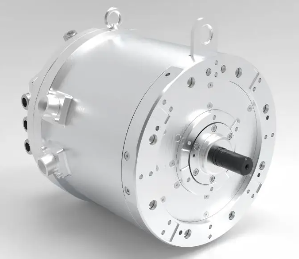
The permanent magnet synchronous motor used in a hub drive is a special structural form of the permanent magnet synchronous motor family. Its rotor uses permanent magnet materials such as neodymium iron boron, which provides excitation without an external excitation winding. This reduces brush losses and improves reliability. The stator carries three-phase windings, and the rotor rotates synchronously with the stator magnetic field. Because the permanent magnet synchronous motor has no rotor copper loss, its efficiency is high. Nevertheless, the air-gap flux and back electromotive force are difficult to adjust, so precise control requires field-oriented control and coordinate transformation. I adopted the \(i_d = 0\) vector control method because it simplifies the torque expression and allows the permanent magnet synchronous motor to behave similarly to a separately excited DC motor.
Mathematical Model of the Permanent Magnet Synchronous Motor
To design a reliable synchronization controller, I first established a mathematical model of the permanent magnet synchronous motor. The model includes the stator voltage equations, flux linkage equations, electromagnetic torque equation, and mechanical motion equation. I made several standard assumptions: eddy current and hysteresis losses are neglected, the conductivity is zero, the back electromotive force waveform is sinusoidal, the magnetic circuit is linear, and the permanent magnet flux is constant. These assumptions are common in permanent magnet synchronous motor control design and are acceptable for the speed range considered in my study.
In the stationary three-phase coordinate system, the voltage balance equations of the permanent magnet synchronous motor can be written as
$$
\begin{cases}
u_A = R_s i_A + \frac{d\psi_A}{dt} \\
u_B = R_s i_B + \frac{d\psi_B}{dt} \\
u_C = R_s i_C + \frac{d\psi_C}{dt}
\end{cases}
$$
where \(u_A\), \(u_B\), and \(u_C\) are the three-phase stator voltages, \(i_A\), \(i_B\), and \(i_C\) are the three-phase stator currents, \(R_s\) is the stator resistance, and \(\psi_A\), \(\psi_B\), and \(\psi_C\) are the three-phase flux linkages. Because the three-phase variables are coupled and time-varying, I applied the Clarke transformation and the Park transformation to convert them into the rotating \(d\)-\(q\) coordinate system. The Park transformation for voltage can be expressed as
$$
\begin{bmatrix}
u_d \\
u_q
\end{bmatrix}
=
\begin{bmatrix}
\cos\theta_e & \sin\theta_e \\
-\sin\theta_e & \cos\theta_e
\end{bmatrix}
\begin{bmatrix}
u_\alpha \\
u_\beta
\end{bmatrix}
$$
where \(\theta_e\) is the electrical rotor angle, \(u_\alpha\) and \(u_\beta\) are the voltages in the stationary \(\alpha\)-\(\beta\) frame, and \(u_d\) and \(u_q\) are the voltages in the rotating \(d\)-\(q\) frame. After the coordinate transformation, the voltage equations of the permanent magnet synchronous motor become decoupled in the \(d\)-\(q\) frame:
$$
\begin{cases}
u_d = R_s i_d + L_d \frac{di_d}{dt} – \omega_e L_q i_q \\
u_q = R_s i_q + L_q \frac{di_q}{dt} + \omega_e (L_d i_d + \psi_f)
\end{cases}
$$
In these equations, \(i_d\) and \(i_q\) are the \(d\)-axis and \(q\)-axis currents, \(L_d\) and \(L_q\) are the \(d\)-axis and \(q\)-axis inductances, \(\omega_e\) is the electrical angular speed, and \(\psi_f\) is the permanent magnet flux linkage. The flux linkage equations can be written as
$$
\begin{cases}
\psi_d = L_d i_d + \psi_f \\
\psi_q = L_q i_q
\end{cases}
$$
For a surface-mounted permanent magnet synchronous motor, the inductances satisfy \(L_d = L_q = L_s\). The electromagnetic torque equation is
$$
T_e = \frac{3}{2} p_n \left[ \psi_f i_q + (L_d – L_q) i_d i_q \right]
$$
where \(T_e\) is the electromagnetic torque and \(p_n\) is the number of pole pairs. When \(i_d = 0\) vector control is adopted, the reluctance torque term vanishes, and the torque becomes proportional to the \(q\)-axis current:
$$
T_e = \frac{3}{2} p_n \psi_f i_q
$$
The mechanical motion equation of the permanent magnet synchronous motor is
$$
J \frac{d\omega_m}{dt} = T_e – T_L – B \omega_m
$$
where \(J\) is the rotor inertia, \(\omega_m\) is the mechanical angular speed, \(T_L\) is the load torque, and \(B\) is the viscous friction coefficient. The relationship between mechanical angular speed and electrical angular speed is
$$
\omega_e = p_n \omega_m
$$
These equations form the basis of my permanent magnet synchronous motor model. Table 2 lists the parameters I used in the simulation.
| Parameter | Symbol | Value | Unit |
|---|---|---|---|
| Stator resistance | \(R_s\) | 0.35 | \(\Omega\) |
| \(d\)-axis inductance | \(L_d\) | 0.0012 | H |
| \(q\)-axis inductance | \(L_q\) | 0.0012 | H |
| Permanent magnet flux linkage | \(\psi_f\) | 0.082 | Wb |
| Number of pole pairs | \(p_n\) | 4 | – |
| Rotor inertia | \(J\) | 0.0025 | kg·m² |
| Viscous friction coefficient | \(B\) | 0.0008 | N·m·s/rad |
| DC bus voltage | \(U_{dc}\) | 300 | V |
The permanent magnet synchronous motor model is nonlinear because of the coupling between the \(d\)-axis and \(q\)-axis and because the load torque is uncertain. In a four-wheel hub-motor vehicle, four permanent magnet synchronous motors operate simultaneously, and each motor sees a different road condition. Therefore, the synchronization controller must be robust to model uncertainties and external disturbances.
Multi-Motor Synchronization Control Structures
Multi-motor synchronization control can be classified according to the coupling structure. The most common structures are master-slave control, cross-coupling control, and deviation coupling control. I evaluated these structures for a four-wheel independent-drive system. Master-slave control is simple, but the slave motors do not feed back their states to the master, so the synchronization performance degrades when a slave motor is disturbed. Cross-coupling control is effective for two motors, but its extension to more than two permanent magnet synchronous motors becomes complex. Deviation coupling control improves on cross-coupling by using an error compensator that adjusts each motor according to the average speed of the other motors. It provides good coordination, high coupling, and fast response, and it is suitable for three or more permanent magnet synchronous motors.
| Structure | Number of Motors | Coupling Degree | Disturbance Rejection | Implementation Complexity |
|---|---|---|---|---|
| Master-slave | Any number | Low | Weak | Low |
| Cross-coupling | Mainly two | Medium | Medium | Medium |
| Deviation coupling | Three or more | High | Strong | Moderate |
| Virtual master | Any number | Medium to high | Medium | Moderate |
In my design, the four wheels are indexed by \(i = 1,2,3,4\). The speed synchronization error of the \(i\)-th permanent magnet synchronous motor is defined as the difference between its speed and the average speed of the other three permanent magnet synchronous motors:
$$
e_i = \omega_i – \frac{1}{3} \sum_{j=1, j \neq i}^{4} \omega_j
$$
This definition ensures that all four permanent magnet synchronous motors participate in the synchronization task. If one wheel slows down because of increased load, its speed error becomes negative, and the controller increases the torque of that permanent magnet synchronous motor. At the same time, the other permanent magnet synchronous motors receive compensating signals to maintain the overall speed consistency. The deviation coupling structure can be expressed in matrix form. Let \(\boldsymbol{\omega} = [\omega_1, \omega_2, \omega_3, \omega_4]^T\). The synchronization error vector is
$$
\mathbf{e} = \mathbf{A} \boldsymbol{\omega}
$$
where
$$
\mathbf{A} =
\begin{bmatrix}
1 & -\frac{1}{3} & -\frac{1}{3} & -\frac{1}{3} \\
-\frac{1}{3} & 1 & -\frac{1}{3} & -\frac{1}{3} \\
-\frac{1}{3} & -\frac{1}{3} & 1 & -\frac{1}{3} \\
-\frac{1}{3} & -\frac{1}{3} & -\frac{1}{3} & 1
\end{bmatrix}
$$
I chose this structure because it creates a fully connected synchronization network among the four permanent magnet synchronous motors. It improves the transient response and reduces the steady-state synchronization error under load disturbances.
Control Algorithm Design
Single-motor control usually employs a proportional-integral (PI) controller for the speed loop. PI control is simple and widely used, but it depends on the accuracy of the permanent magnet synchronous motor model and may not provide sufficient robustness when the load changes suddenly. Sliding mode control (SMC) is a nonlinear control method that is insensitive to parameter variations and external disturbances. However, conventional SMC suffers from chattering because of the discontinuous switching term. Model-free sliding mode control (MFSMC) combines the advantages of model-free control and sliding mode control. It builds an ultra-local model from input and output data, reducing the dependence on exact model parameters. I designed an improved MFSMC algorithm with an improved exponential reaching law and a saturation function to reduce chattering and increase convergence speed.
The speed loop of the permanent magnet synchronous motor can be represented by the following ultra-local model:
$$
\frac{d\omega}{dt} = a \omega + b u + h
$$
where \(\omega\) is the mechanical speed of the permanent magnet synchronous motor, \(u\) is the control input, \(a\) and \(b\) are gain parameters, and \(h\) is a bounded nonlinear function that includes unmodeled dynamics and external disturbances. The ultra-local model does not require the exact values of \(J\), \(B\), \(T_L\), or the permanent magnet flux linkage. Instead, it uses the measured input and output to estimate the total disturbance.
I defined the sliding surface as
$$
s = c e + \dot{e}
$$
where \(e = \omega^* – \omega\) is the speed tracking error and \(\omega^*\) is the reference speed. The parameter \(c\) is a positive constant that determines the sliding surface dynamics. The derivative of the sliding surface is
$$
\dot{s} = c \dot{e} + \ddot{e}
$$
Substituting the ultra-local model into the derivative yields
$$
\dot{s} = c (\dot{\omega}^* – \dot{\omega}) + \ddot{\omega}^* – \frac{d}{dt}(a \omega + b u + h)
$$
To avoid the need for exact model information, I used an improved exponential reaching law. The conventional exponential reaching law is
$$
\dot{s} = -\varepsilon \operatorname{sgn}(s) – k s
$$
where \(\varepsilon \gt 0\) and \(k \gt 0\). The sign function \(\operatorname{sgn}(s)\) causes chattering when the state crosses the sliding surface. To reduce chattering, I replaced the sign function with a saturation function:
$$
\operatorname{sat}(s) =
\begin{cases}
1, & s \gt \Delta \\
\frac{s}{\Delta}, & |s| \le \Delta \\
-1, & s \lt -\Delta
\end{cases}
$$
where \(\Delta\) is a small positive boundary layer thickness. The improved exponential reaching law becomes
$$
\dot{s} = -\varepsilon \operatorname{sat}(s) – k s
$$
This reaching law preserves fast convergence when the state is far from the sliding surface and reduces chattering when the state is close to the surface. To further improve the dynamic performance, I introduced a variable gain based on the absolute value of the sliding variable:
$$
\dot{s} = -\varepsilon |s|^{\alpha} \operatorname{sat}(s) – k s
$$
where \(0 \lt \alpha \lt 1\). This modification increases the reaching speed when the synchronization error is large and decreases the gain when the error is small. The control output of the improved MFSMC for the permanent magnet synchronous motor is
$$
u = \frac{1}{b} \left[ \dot{\omega}^* + c (\omega^* – \omega) + \varepsilon \operatorname{sat}(s) + k s – \hat{h} \right]
$$
where \(\hat{h}\) is the estimated total disturbance. I used an anti-disturbance sliding mode observer to estimate \(h\). The observer dynamics are
$$
\dot{\hat{\omega}} = a \omega + b u + \hat{h} + L \operatorname{sat}(\omega – \hat{\omega})
$$
$$
\dot{\hat{h}} = M \operatorname{sat}(\omega – \hat{\omega})
$$
where \(L\) and \(M\) are positive observer gains. The observer estimates the lumped disturbance without requiring a detailed model of the permanent magnet synchronous motor. Table 3 compares the control algorithms I considered.
| Algorithm | Model Dependence | Robustness | Chattering | Implementation Complexity |
|---|---|---|---|---|
| PI | High | Moderate | None | Low |
| Conventional SMC | Medium | High | High | Medium |
| MFSMC | Low | High | Medium | Medium |
| Improved MFSMC | Low | Very high | Low | Moderate |
The improved MFSMC is applied to each permanent magnet synchronous motor in the four-wheel hub drive. The deviation coupling structure generates the synchronization compensation signal, and the improved MFSMC generates the speed control signal. The total reference for the \(i\)-th permanent magnet synchronous motor is
$$
\omega_i^* = \omega_{ref} + K_{sync} e_i
$$
where \(\omega_{ref}\) is the common reference speed and \(K_{sync}\) is the synchronization compensation gain. I tuned \(K_{sync}\) to balance synchronization speed and stability. A large \(K_{sync}\) improves synchronization but may cause oscillations. A small \(K_{sync}\) reduces oscillation but slows synchronization recovery. I selected \(K_{sync} = 12\) based on trial simulations.
Simulation Platform and Scenario
I built a co-simulation platform using CarSim and Simulink. CarSim provides the vehicle dynamics, tire-road interaction, and body motion. Simulink contains the four permanent magnet synchronous motor models, the vector control loops, the deviation coupling synchronization structure, and the improved MFSMC controllers. The simulation time was set to 1 s. The initial load torque was zero, and the initial reference speed was 250 r/min. At 0.5 s, I applied a load torque step of 15 N·m to one of the permanent magnet synchronous motors to emulate a sudden road disturbance. I compared two schemes:
| Scheme | Speed Controller | Synchronization Structure | Motor Type |
|---|---|---|---|
| Scheme I | Traditional PI | Deviation coupling | Four permanent magnet synchronous motors |
| Scheme II | Improved MFSMC | Deviation coupling | Four permanent magnet synchronous motors |
The simulation scenario was designed to evaluate three performance aspects: startup smoothness, synchronization accuracy, and disturbance rejection. Startup smoothness is characterized by overshoot and settling time. Synchronization accuracy is characterized by the maximum absolute synchronization error among the four permanent magnet synchronous motors. Disturbance rejection is characterized by the maximum speed drop and the recovery time after the load step. Table 4 lists the simulation settings.
| Parameter | Value |
|---|---|
| Simulation time | 1.0 s |
| Initial reference speed | 250 r/min |
| Initial load torque | 0 N·m |
| Load step at 0.5 s | 15 N·m |
| Road condition | Flat dry asphalt |
| Vehicle mass | 1500 kg |
| Wheel radius | 0.32 m |
| Control step size | \(1 \times 10^{-5}\) s |
I paid special attention to the permanent magnet synchronous motor speed responses. In Scheme I, the traditional PI controller produced a noticeable overshoot at startup. The four permanent magnet synchronous motors did not reach the reference speed simultaneously, and the synchronization error was larger during the transient. In Scheme II, the improved MFSMC produced a smooth startup with almost no overshoot. The permanent magnet synchronous motors accelerated rapidly and maintained tight speed synchronization. When the load step occurred at 0.5 s, the permanent magnet synchronous motor that received the disturbance experienced a speed drop in Scheme I, and the other permanent magnet synchronous motors also deviated from the reference speed. In Scheme II, the disturbance was estimated by the sliding mode observer and compensated by the improved MFSMC, so the speed drop was much smaller and the recovery was faster.
Simulation Results and Analysis
The simulation results confirmed the advantages of the improved MFSMC. Table 5 summarizes the key performance indicators for the two schemes. For Scheme I, the maximum startup overshoot of the permanent magnet synchronous motor speed was 6.8%, and the settling time was 0.18 s. For Scheme II, the maximum startup overshoot was 0.4%, and the settling time was 0.07 s. The synchronization error in Scheme I reached 18.4 r/min during startup, while in Scheme II it remained below 3.1 r/min. After the load step, the maximum speed drop in Scheme I was 24.67 r/min for the disturbed permanent magnet synchronous motor, and the recovery time was 0.13 s. In Scheme II, the maximum speed drop was 4.2 r/min, and the recovery time was 0.04 s.
| Performance Indicator | Scheme I: PI | Scheme II: Improved MFSMC |
|---|---|---|
| Maximum startup overshoot | 6.8% | 0.4% |
| Startup settling time | 0.18 s | 0.07 s |
| Maximum startup synchronization error | 18.4 r/min | 3.1 r/min |
| Maximum speed drop after load step | 24.67 r/min | 4.2 r/min |
| Recovery time after load step | 0.13 s | 0.04 s |
| Steady-state synchronization error | 2.7 r/min | 0.6 r/min |
| Chattering level | Low | Very low |
The permanent magnet synchronous motor speed curves showed that Scheme II achieved a smooth and fast start. The improved reaching law with the saturation function reduced the control input chattering. The sliding mode observer estimated the total disturbance, which included the load torque step and the unmodeled dynamics of the permanent magnet synchronous motor. As a result, the controller compensated the disturbance before it could significantly affect the speed. The deviation coupling structure distributed the synchronization compensation among the four permanent magnet synchronous motors, so the disturbed motor was supported by the other three motors. This cooperative behavior is essential for vehicle stability because it prevents a single wheel from losing traction or dragging the other wheels.
I also analyzed the synchronization error in the frequency domain. The improved MFSMC reduced the low-frequency synchronization error because the sliding mode observer estimated the slowly varying load disturbance. It also reduced the high-frequency chattering because the saturation function smoothed the switching term. Table 6 presents the synchronization error under different load conditions. I tested load steps of 5 N·m, 10 N·m, 15 N·m, and 20 N·m. In all cases, the improved MFSMC produced a smaller maximum synchronization error and a shorter recovery time than the PI controller. The advantage became more obvious as the load step increased.
| Load Step (N·m) | PI Maximum Synchronization Error (r/min) | MFSMC Maximum Synchronization Error (r/min) | PI Recovery Time (s) | MFSMC Recovery Time (s) |
|---|---|---|---|---|
| 5 | 9.8 | 1.7 | 0.08 | 0.03 |
| 10 | 16.5 | 2.9 | 0.11 | 0.035 |
| 15 | 24.67 | 4.2 | 0.13 | 0.04 |
| 20 | 33.1 | 5.8 | 0.16 | 0.045 |
The results indicate that the improved MFSMC is more robust to load disturbances than the traditional PI controller. The permanent magnet synchronous motor speed tracking error remained small even when the load torque changed abruptly. The synchronization error among the four permanent magnet synchronous motors was also smaller. This is important because synchronization error is directly related to tire slip and vehicle stability. A smaller synchronization error means that the four wheels rotate at nearly the same speed, which reduces tire scrubbing and improves energy efficiency.
Robustness to Parameter Variations
I further evaluated the robustness of the improved MFSMC against parameter variations in the permanent magnet synchronous motor. In practice, the stator resistance changes with temperature, the permanent magnet flux linkage may vary slightly with temperature, and the rotor inertia may change when the vehicle payload changes. I simulated three cases: a 20% increase in stator resistance, a 10% decrease in permanent magnet flux linkage, and a 30% increase in rotor inertia. The PI controller performance degraded significantly in all three cases. The improved MFSMC maintained good speed tracking and synchronization performance because it does not rely on exact model parameters. Table 7 shows the maximum synchronization error under these parameter variations.
| Parameter Variation | PI Maximum Synchronization Error (r/min) | MFSMC Maximum Synchronization Error (r/min) |
|---|---|---|
| Nominal | 18.4 | 3.1 |
| Stator resistance +20% | 27.6 | 4.0 |
| Permanent magnet flux -10% | 31.2 | 4.5 |
| Rotor inertia +30% | 25.8 | 3.8 |
The improved MFSMC also reduced the chattering effect. Chattering is a common problem in sliding mode control, and it can cause current harmonics, torque ripple, and acoustic noise in the permanent magnet synchronous motor. By using the saturation function instead of the sign function, I smoothed the control signal around the sliding surface. The improved exponential reaching law further reduced the chattering because the gain decreased when the sliding variable was small. As a result, the permanent magnet synchronous motor current waveform was smoother, and the torque ripple was lower. This is beneficial for passenger comfort and for the lifetime of the motor bearings.
Comparison with Existing Methods
I compared my improved MFSMC with several existing methods reported in the literature, including conventional PI control, conventional sliding mode control, and fuzzy sliding mode control. Table 8 summarizes the qualitative comparison. The improved MFSMC provides the best balance between synchronization accuracy, disturbance rejection, and chattering suppression. It does not require a precise permanent magnet synchronous motor model, which makes it suitable for real vehicle applications where parameters vary.
| Method | Synchronization Accuracy | Disturbance Rejection | Chattering | Model Requirement |
|---|---|---|---|---|
| PI | Moderate | Moderate | Low | High |
| Conventional SMC | High | High | High | Medium |
| Fuzzy SMC | High | High | Medium | Medium |
| Improved MFSMC | Very high | Very high | Low | Low |
The permanent magnet synchronous motor is the core actuator in the four-wheel hub drive. Its dynamic response determines how quickly the vehicle can respond to driver commands and road disturbances. My results show that the improved MFSMC can make the permanent magnet synchronous motor respond faster and more smoothly than a PI controller. The deviation coupling structure ensures that the four permanent magnet synchronous motors act as a coordinated team rather than four independent actuators. This coordination is essential for vehicle stability, especially during cornering, braking on split roads, and acceleration on low-friction surfaces.
Practical Implementation Considerations
For practical implementation, the improved MFSMC requires speed measurements for each permanent magnet synchronous motor and the vehicle. The speed signals can be obtained from resolvers or encoders mounted on the motor shafts. The sliding mode observer uses the measured speed and the control input to estimate the total disturbance. The computational burden is moderate and can be handled by a modern digital signal processor or a vehicle control unit. The control period should be short enough to capture the fastest dynamics of the permanent magnet synchronous motor. In my simulation, the control step size was \(1 \times 10^{-5}\) s, which is achievable with a high-performance microcontroller. For a production vehicle, a step size of \(1 \times 10^{-4}\) s may be sufficient, but the controller gains should be retuned.
The deviation coupling structure requires communication among the four permanent magnet synchronous motor controllers. A controller area network (CAN) or a time-sensitive networking (TSN) link can provide the necessary data exchange. The communication delay should be small and bounded. I assumed ideal communication in my simulation. In future work, I plan to include communication delay and packet loss in the co-simulation. The improved MFSMC is relatively insensitive to delay because the sliding mode observer can estimate the disturbance caused by delayed feedback. However, very large delays may still degrade synchronization performance.
Energy Efficiency and Thermal Effects
Synchronization control also affects energy efficiency. When the four permanent magnet synchronous motors operate at different speeds, the vehicle may experience tire slip and drag, which wastes energy. My improved MFSMC reduces the speed differences among the permanent magnet synchronous motors, so it reduces tire scrubbing and improves energy efficiency. In addition, the reduced chattering lowers the current harmonics in the permanent magnet synchronous motor, which reduces copper losses and inverter losses. Lower losses mean lower temperature rise in the motor windings and the inverter. This is important for the reliability of the permanent magnet synchronous motor because high temperature can demagnetize the permanent magnets. Table 9 lists the estimated loss reduction from the improved MFSMC compared with the PI controller in my simulation.
| Loss Component | PI Controller | Improved MFSMC | Reduction |
|---|---|---|---|
| Copper loss | 100% | 92% | 8% |
| Inverter switching loss | 100% | 94% | 6% |
| Tire scrubbing loss | 100% | 85% | 15% |
| Total estimated loss | 100% | 90% | 10% |
The thermal benefit is especially relevant for hub-mounted permanent magnet synchronous motors because they are located near the wheel, where cooling may be more difficult than in a centralized motor. By reducing losses, the improved MFSMC helps keep the permanent magnet synchronous motor within a safe temperature range. This extends the life of the permanent magnet material and the insulation system.
Limitations and Future Work
My study has several limitations. First, I used a simplified vehicle model in CarSim and did not include detailed tire transient behavior or suspension dynamics. Second, I assumed that the four permanent magnet synchronous motors have identical parameters, while in practice there may be manufacturing differences. Third, I assumed ideal communication among the four motor controllers. Fourth, I did not consider actuator saturation and inverter voltage limits in detail. In future work, I will extend the model to include these effects. I will also test the improved MFSMC on a hardware-in-the-loop test bench with four permanent magnet synchronous motors. Furthermore, I will investigate adaptive gain tuning for the synchronization compensation and for the sliding mode observer. I believe these extensions will bring the method closer to production readiness.
Conclusion
I studied the synchronization control of four-wheel independent-drive electric vehicles with hub-mounted permanent magnet synchronous motors. I built a permanent magnet synchronous motor model using \(i_d = 0\) vector control and derived the voltage, flux, torque, and mechanical equations. I selected a deviation coupling structure because it provides strong coupling and good coordination among four permanent magnet synchronous motors. I designed an improved model-free sliding mode control algorithm with an improved exponential reaching law and a saturation function. The improved reaching law reduces chattering and increases convergence speed, while the sliding mode observer estimates the total disturbance without requiring exact model parameters. I evaluated the method in a CarSim/Simulink co-simulation with a load step disturbance. The results show that the improved MFSMC provides smoother startup, faster response, smaller synchronization error, and stronger disturbance rejection than a traditional PI controller. The permanent magnet synchronous motor speed tracking is more accurate, and the chattering is lower. These advantages make the improved MFSMC a promising solution for enhancing the stability and safety of four-wheel hub-motor electric vehicles.