
In this study, I design, model, and experimentally validate an active cooling architecture for a PMSM electric motor operating at high power density. My motivation comes from a simple observation that repeats itself across every traction platform I have examined: the PMSM electric motor is thermally limited long before it is electromagnetically limited. When I push a modern traction machine toward its peak torque envelope, the stator winding, the stator core, and the permanent magnets accumulate heat faster than a conventional single-loop liquid cooling circuit can remove it. The consequences are not merely a derating event. Excessive temperature in a PMSM electric motor accelerates insulation aging, reduces coercivity in the permanent magnets, and eventually produces irreversible demagnetization. I therefore treat thermal management not as an accessory to the electric drive, but as a first-order design discipline that determines the usable power density of the PMSM electric motor.
My central thesis is that no single cooling mechanism is sufficient for a contemporary PMSM electric motor. Liquid cooling is excellent for continuous, large-area heat removal, but it cannot reach the rotating rotor or the interior of the winding bundle. Oil cooling can reach those internal hot spots, yet its sealing complexity and mass penalty make it unattractive as a sole solution. Phase-change cooling absorbs transient heat spikes without any pumping power, but its thermal capacitance is finite and requires periodic recharge. I therefore combine these mechanisms into a multimodal coupled system in which the stator, the rotor, and the controller each receive a cooling path tailored to its own thermal signature. The coordination of those paths is handled by a long short-term memory network that predicts the thermal trajectory of the PMSM electric motor and allocates cooling capacity ahead of the load transient rather than after it.
Thermal Sources and Cooling Demand in the Electric Drive
Before I can design a cooling system, I must quantify where the heat is generated inside a PMSM electric motor. The dominant loss mechanisms are copper loss in the stator winding, iron loss in the laminated core, eddy-current loss in the permanent magnets, and mechanical loss in the bearings and rotor. I summarize the principal heat sources I use as design inputs in Table 1.
| Component | Dominant heat source | Share of total loss | Temperature-sensitive point and failure risk |
|---|---|---|---|
| PMSM electric motor | Stator copper loss, core eddy-current loss | 60%–70% | Permanent magnet above 150 °C: demagnetization; winding insulation aging |
| Motor controller | Switching and conduction loss of IGBT or MOSFET devices | 20%–30% | Junction temperature above 175 °C: breakdown |
| Reducer | Gear meshing friction, bearing loss | 10%–15% | Lubricant above 140 °C: film failure |
For the PMSM electric motor itself, I express the copper loss of the three-phase winding as
$$ P_{cu} = m I_{rms}^{2} R_{ac} \left(1 + \alpha \left(T_w – T_0\right)\right) $$
where \(m\) is the number of phases, \(I_{rms}\) is the root-mean-square phase current, \(R_{ac}\) is the alternating-current resistance of the winding, \(\alpha\) is the temperature coefficient of copper, \(T_w\) is the winding temperature, and \(T_0\) is the reference temperature. The temperature dependence in this expression is the reason my control strategy cannot be open loop: as the winding heats up, its resistance rises, the copper loss rises, and the thermal runaway margin shrinks.
The iron loss in the stator core is represented by the classical three-term separation:
$$ P_{fe} = k_h f B^{n} + k_e f^{2} B^{2} + k_a f^{1.5} B^{1.5} $$
where \(k_h\), \(k_e\), and \(k_a\) are the hysteresis, eddy-current, and anomalous loss coefficients, \(f\) is the electrical frequency, \(B\) is the peak flux density, and \(n\) is the Steinmetz exponent. In a PMSM electric motor with a high pole count, the electrical frequency at top speed can be several hundred hertz, so the eddy-current term becomes a substantial fraction of the total loss. This is why I place the highest thermal conductivity material directly against the stator lamination stack rather than somewhere in the housing.
The permanent-magnet eddy-current loss is smaller in absolute terms but thermally more dangerous, because the magnets are buried inside the rotor where the heat path to any coolant is long. I estimate it as
$$ P_{mag} = \frac{\pi^{2} \sigma_{m} d_{m}^{2} f^{2} B_{m}^{2} V_{m}}{6 \rho_{m}} $$
where \(\sigma_{m}\) is the electrical conductivity of the magnet, \(d_{m}\) is the magnet segment thickness, \(B_{m}\) is the local flux density, \(V_{m}\) is the magnet volume, and \(\rho_{m}\) is the magnet density. The strong \(f^{2}\) dependence tells me that a PMSM electric motor at high speed produces magnet heat that the rotor cooling path must be able to remove directly. Conduction across the air gap alone is not an adequate strategy.
Why Multimodal Coupling Is Necessary
I compared the mainstream cooling options available for a PMSM electric motor and recorded their respective roles in a coupled architecture. The result of that comparison is given in Table 2. What becomes clear to me is that each mechanism occupies a different region of the thermal design space.
| Cooling mechanism | Principle | Advantage | Limitation | Role in the multimodal system |
|---|---|---|---|---|
| Liquid cooling | Coolant flows through a channel and carries heat away | High heat transfer coefficient, controllable cost | Cannot directly cool internal hot spots | Base continuous heat-removal path |
| Oil cooling | Oil contacts the heat-generating component directly | Direct hot-spot cooling, large temperature drop | Sealing complexity, mass and cost penalty | Dedicated rotor and internal winding path |
| Phase-change cooling | Latent heat absorption during phase transition | Zero pumping power, suppresses transient spikes | Finite thermal capacity, requires recharge | Thermal buffer and peak-temperature clipping |
| Air cooling | Forced convection to ambient air | Simple structure, low cost | Low heat transfer efficiency | Auxiliary path for low-power operation |
The principle I adopt is therefore spatial and temporal complementarity. Spatially, the stator receives a layered conduction path because its loss is distributed over a large area and must be removed continuously. The rotor receives a direct-contact oil path because its loss is concentrated in a small, rotating volume that is difficult to reach by conduction. Temporally, the phase-change layer absorbs the fast transient that a liquid loop cannot follow, while the liquid loop removes the steady component. I can write the overall energy balance of the coupled system as
$$ Q_{total} = Q_{stator} + Q_{rotor} + Q_{pcm} = \dot{m}_{c} c_{p,c} \Delta T_{c} + \dot{m}_{o} c_{p,o} \Delta T_{o} + m_{pcm} L_{f} $$
where \(\dot{m}_{c}\) and \(\dot{m}_{o}\) are the coolant and oil mass flow rates, \(c_{p,c}\) and \(c_{p,o}\) are their specific heat capacities, \(\Delta T_{c}\) and \(\Delta T_{o}\) are the temperature rises across the respective loops, \(m_{pcm}\) is the mass of phase-change material, and \(L_{f}\) is its latent heat of fusion. This single equation is the backbone of my control allocation logic.
Stator Layered Cooling Structure
I designed the stator housing as a three-layer composite. The inner layer is a nanoporous ceramic thermally conductive layer with a porosity of approximately 70%, built from a silicon carbide or aluminum nitride skeleton. Its anisotropic thermal conductivity conducts heat radially away from the lamination stack and the end winding. The high melting point of aluminum nitride, combined with the nanopore structure that suppresses sintering shrinkage at elevated temperature, keeps the pore network stable over the life of the PMSM electric motor. Table 3 lists the skeleton materials I evaluated.
| Material system | Solid-phase thermal conductivity (dense state) / (W·m⁻¹·K⁻¹) | Characteristics and application considerations |
|---|---|---|
| SiC | 120–270 | Good high-temperature stability, moderate cost |
| AlN | 200–320 | Extremely high thermal conductivity, requires oxidation protection |
| ZrB₂/SiC composite ceramic | 60–100 | Ultra-high-temperature stability, suitable for extreme environments |
The middle layer is a graphene-based phase-change material. The graphene flakes, each approximately 0.335 nm thick, form a three-dimensional percolating network inside the matrix, which raises the effective thermal conductivity by one to two orders of magnitude. The nanoconfinement effect, in which graphene encapsulates the paraffin molecules and reduces intermolecular void space, suppresses leakage during melting and improves structural stability. I selected a phase-change point near 65 °C and a latent heat of at least 250 kJ/kg so that the layer buffers the temperature of the PMSM electric motor during short overload events. Table 4 compares the graphene-based material with a conventional paraffin phase-change material.
| Property | Conventional paraffin PCM | Graphene-based PCM | Improvement |
|---|---|---|---|
| Thermal conductivity / (W·m⁻¹·K⁻¹) | 0.2–0.3 | 5–15 | 20× to 50× |
| Latent heat / (kJ·kg⁻¹) | 180–220 | ≥250 | 15%–30% |
| Thermal response speed | Slow | Fast, 40% shorter response time | Better transient handling |
| Cycling stability | More than 20% degradation after 500 cycles | Less than 5% degradation after 1 000 cycles | Significantly extended life |
The outer layer is a double-helix microchannel liquid-cooling plate with a channel width of only 0.5 mm. The double-helix geometry forces the coolant to sweep the entire outer circumference of the stator rather than following a short parallel path, which increases the effective heat-transfer area and reduces the maximum local temperature of the PMSM electric motor. I express the convective heat transfer in the microchannel as
$$ Q_{conv} = h A_{s} \left(T_{wall} – T_{coolant}\right) $$
with the Nusselt number in the laminar microchannel regime approximated by
$$ Nu = \frac{h D_{h}}{k_{c}} = 4.36 + \frac{0.065 \left(D_{h}/L\right) Re\,Pr}{1 + 0.04 \left[\left(D_{h}/L\right) Re\,Pr\right]^{2/3}} $$
where \(D_{h}\) is the hydraulic diameter, \(L\) is the channel length, \(Re\) is the Reynolds number, \(Pr\) is the Prandtl number, and \(k_{c}\) is the coolant thermal conductivity. The small hydraulic diameter of my channel keeps the flow in the thermally developing regime, which is precisely where the heat transfer coefficient is highest.
For the coolant itself, I disperse 1.5 wt% boron nitride nanosheets into a conventional 50:50 water–glycol mixture. The nanosheets are electrically insulating and highly anisotropic in thermal conductivity, and their addition raises the effective thermal conductivity of the coolant by approximately 35%. I estimate the mixture conductivity with the Maxwell–Garnett effective medium expression:
$$ \frac{k_{eff}}{k_{bf}} = \frac{k_{p} + 2k_{bf} + 2\phi \left(k_{p} – k_{bf}\right)}{k_{p} + 2k_{bf} – \phi \left(k_{p} – k_{bf}\right)} $$
where \(k_{bf}\) is the base-fluid conductivity, \(k_{p}\) is the particle conductivity, and \(\phi\) is the particle volume fraction. This modified coolant is what allows the outer microchannel layer to remove both the heat released by the phase-change layer and the heat conducted directly through the ceramic skeleton.
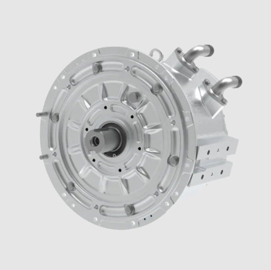
Rotor Dual-Path Cooling Structure
The rotor of a high-speed PMSM electric motor is the most difficult region to cool because it rotates and because the heat path to the housing is interrupted by the air gap. I therefore designed a dual-path scheme that combines forced convection through an axial oil channel with evaporative cooling from a radial spray.
In the axial path, a minimal-quantity lubrication nozzle embedded in the housing delivers oil directly to the rotor with a precisely controlled flow between 0.2 mL/s and 1.5 mL/s. This flow both cools the rotor and improves bearing lubrication, which is a useful secondary benefit. In the radial path, laser-etched micro-holes of 50 µm diameter are distributed on the rotor surface. Centrifugal force atomizes the oil into fine droplets that impinge on the rotor surface and increase the effective heat-transfer area without adding aerodynamic drag.
The oil circuit is a closed loop. The pump draws oil from the reservoir, passes it through a filter, and delivers it under pressure to a rotary union. A three-way valve splits the flow between the central oil channel of the hollow shaft and the housing nozzle gallery. The shaft nozzle injects oil into the hollow shaft, from which centrifugal action drives it through the micro-holes. The housing nozzle sprays oil onto the rotor surface. After absorbing heat, part of the oil evaporates and the remainder is thrown outward by centrifugal force to the inner wall of the housing. The oil mist and droplets collect at the bottom of the housing and return through a pipe to the reservoir, where an oil cooler rejects the heat to the vehicle cooling loop.
The centrifugal atomization condition at the rotor surface can be expressed through the balance between surface tension and centrifugal pressure:
$$ \rho_{o} \omega^{2} r_{o} d_{p} \geq \frac{4 \sigma_{o}}{d_{p}} $$
where \(\rho_{o}\) is the oil density, \(\omega\) is the angular velocity, \(r_{o}\) is the rotor radius, \(d_{p}\) is the droplet diameter, and \(\sigma_{o}\) is the oil surface tension. When this inequality is satisfied, the oil film breaks into droplets that can penetrate the boundary layer and reach the magnet-retaining sleeve. I use this relation to select the micro-hole diameter and the minimum rotor speed at which the radial path becomes fully effective.
The heat removed by the rotor oil path is
$$ Q_{rotor} = \dot{m}_{o} \left[ c_{p,o} \left(T_{out} – T_{in}\right) + x_{v} h_{fg} \right] $$
where \(x_{v}\) is the vapor mass fraction generated by flash evaporation and \(h_{fg}\) is the latent heat of vaporization. The presence of the second term is important because it means the rotor path can remove a large amount of heat with a small oil flow, which keeps the auxiliary power consumption of the PMSM electric motor low.
System Architecture and Operating Sequence
The complete cooling system is coordinated by a controller integrated into the motor control unit. The sequence for the stator and oil-cooler loop is as follows. A stator temperature sensor measures the stator temperature and transmits it to the controller. The controller computes the cooling demand and passes it to the vehicle control unit. The vehicle control unit commands the coolant pump to deliver the requested flow, and the controller positions the three-way valve to distribute flow between the stator microchannel plate and the oil cooler.
The rotor loop operates in parallel. A rotor temperature sensor transmits the rotor temperature to the controller. The controller computes the required oil flow, starts the oil pump, and positions a second three-way valve to split the oil between the axial channel and the radial spray path. Because the two loops share the same controller, the allocation between them can be changed within a single control cycle, which is what makes the architecture genuinely multimodal rather than merely multi-circuit.
Intelligent Thermal Management and Coordinated Control
The supervisory architecture forms a closed loop of sensing, prediction, decision, and execution. Multi-source sensors provide temperature, current, speed, and vehicle signals. The core controller uses a long short-term memory temperature prediction model as a feed-forward brain and a multi-objective optimizer as the decision center. It then coordinates the coolant pump, the oil pump, and the valves to regulate the temperature of the PMSM electric motor with high precision and low auxiliary power.
Data Preparation and Feature Engineering
I fuse controller area network bus data with high-sampling-rate sensor data acquired at 10 Hz or faster. The key features are the direct-axis and quadrature-axis currents \(I_d\) and \(I_q\), the rotor speed \(n\), the direct-current bus voltage \(U_{dc}\), the historical temperature sequence of the stator winding \(T_s\), the rotor \(T_r\), and the coolant inlet \(T_{in}\), together with vehicle-level signals such as vehicle speed \(v\) and accelerator pedal opening \(A_{cc}\). I preprocess the data with a sliding time window to construct supervised learning samples, and I normalize each input according to
$$ x_{norm} = \frac{x – x_{min}}{x_{max} – x_{min}} $$
I also apply an isolation forest algorithm to detect and remove outliers so that the training set reflects genuine thermal behavior rather than sensor faults.
Long Short-Term Memory Network Construction
I designed a two-layer stacked long short-term memory network to balance expressive power and computational efficiency on an embedded controller. The input layer receives a sequence of length \(L\), equal to 60 time steps, which corresponds to one minute of historical data. The first long short-term memory layer contains 64 neurons and returns the full sequence, which allows it to capture high-level temporal patterns. A dropout layer with a rate of 0.2 follows it to prevent overfitting. The second long short-term memory layer contains 32 neurons and returns only the final time-step output, which aggregates the sequence into a compact representation. A fully connected output layer produces the predicted temperatures for the next \(P\) time steps, equal to 10 steps, corresponding to a 10 s horizon. Table 5 summarizes the configuration.
| Layer | Configuration | Purpose |
|---|---|---|
| Input | 60 time steps, multi-feature sequence | Accepts historical thermal and electrical signals |
| LSTM layer 1 | 64 neurons, full sequence returned | Captures high-level temporal patterns |
| Dropout | Rate 0.2 | Suppresses overfitting |
| LSTM layer 2 | 32 neurons, final step only | Aggregates information into a compact state |
| Fully connected output | 10 future time steps | Predicts the thermal trajectory of the PMSM electric motor |
The internal gate equations of each long short-term memory cell are
$$ i_t = \sigma\left(W_i \left[h_{t-1}, x_t\right] + b_i\right) $$
$$ f_t = \sigma\left(W_f \left[h_{t-1}, x_t\right] + b_f\right) $$
$$ o_t = \sigma\left(W_o \left[h_{t-1}, x_t\right] + b_o\right) $$
$$ \tilde{C}_t = \tanh\left(W_C \left[h_{t-1}, x_t\right] + b_C\right) $$
$$ C_t = f_t \odot C_{t-1} + i_t \odot \tilde{C}_t $$
$$ h_t = o_t \odot \tanh\left(C_t\right) $$
where \(i_t\), \(f_t\), and \(o_t\) are the input, forget, and output gates, \(C_t\) is the cell state, \(h_t\) is the hidden state, \(W\) and \(b\) are trainable weights and biases, \(\sigma\) is the logistic sigmoid, and \(\odot\) denotes the Hadamard product. The cell state is what allows the network to retain thermal history over long horizons, which is essential because the thermal time constant of a PMSM electric motor is much longer than the electrical time constant.
Model Training and Deployment
I train the network on a historical driving dataset that covers urban, suburban, and highway operation, split into 70% training, 15% validation, and 15% test partitions. I use the Adam optimizer with the root mean square error as the loss function:
$$ RMSE = \sqrt{\frac{1}{N}\sum_{i=1}^{N}\left(y_i – \hat{y}_i\right)^{2}} $$
On the test set, the mean absolute error of the hot-spot temperature prediction over a 10 s horizon stays within ±1.5 °C, which satisfies the precision required by the controller. After training, I quantize and prune the model so that it can be deployed on the vehicle domain controller for millisecond-level online inference.
Prediction-Based Multi-Parameter Coordinated Control
The core task of the controller is to convert the predicted temperatures into optimal commands for the cooling actuators. I use a hierarchical coordination method. The upper layer is a multi-objective optimization decision maker. It takes the predicted temperature trajectory from the long short-term memory network, the current efficiency map of the PMSM electric motor, and the auxiliary power models of the pumps, and it solves a receding-horizon optimization problem within each control period. The cost function is
$$ J = \sum_{k=1}^{P} w_1 \left(T_{pred,k} – T_{target}\right)^{2} + w_2 P_{pump} + w_3 P_{oil\_pump} $$
where \(T_{target}\) is the temperature of the optimal efficiency region, typically around 80 °C, \(P_{pump}\) and \(P_{oil\_pump}\) are the predicted powers of the coolant pump and the oil pump, and \(w_1\), \(w_2\), and \(w_3\) are weights that I adjust according to the driving mode. In a sport mode I increase \(w_1\) so that performance dominates; in an economy mode I increase \(w_2\) and \(w_3\) so that auxiliary energy consumption dominates. The optimizer outputs the total heat rejection \(Q_{rep}\) expected over the horizon and the optimal split ratio \(k\) between the stator loop and the rotor loop:
$$ k = \frac{Q_{stator}}{Q_{total}} $$
The lower layer is a multi-actuator coordinated controller. It converts the total heat rejection and the split ratio into concrete commands and trims them with feedback. For the stator loop,
$$ Q_{stator,rep} = k Q_{rep} $$
and from the coolant temperature difference I compute the required flow \(F_{coolant}\). I then query the flow–power characteristic of the electronically controlled pump and issue the optimal speed command, which can be either a three-step discrete command of 2, 4, or 6 L/min or a stepless command for finer regulation. For the rotor loop,
$$ Q_{rotor,rep} = \left(1 – k\right) Q_{rep} $$
and together with the predicted rotor temperature I decide whether the axial path or the radial spray path should dominate. I adjust the pulse-width modulation frequency of the electronic oil pump between 1 kHz and 10 kHz and the proportional valve opening to control the injection pressure and flow between 0.2 mL/s and 1.5 mL/s.
I also coordinate the phase-change material state. By monitoring whether the layer is solid, in transition, or fully liquid, I can deliberately reduce the liquid cooling intensity slightly when a large power pulse is predicted, so that the phase-change layer absorbs the peak and the instantaneous pump power stays low. This is a small but meaningful contribution to the overall energy efficiency of the electric drive, and it is only possible because the controller has a prediction of the thermal trajectory of the PMSM electric motor rather than a simple feedback error.
Failure Protection and Safety Redundancy
If the prediction error persists above a threshold, the system switches automatically to a robust backup controller based on reinforcement-learning rules. The critical loops, including the main coolant pump and the main oil pump, use dual redundancy. When a fault is detected, the controller switches to the backup circuit within milliseconds and transitions to a safe, performance-limited cooling mode that satisfies the Automotive Safety Integrity Level C requirement. I consider this layer mandatory for any thermal architecture that will be deployed on a road vehicle, because the cost of a cooling failure in a high-power-density PMSM electric motor is a stator winding short or a permanent-magnet demagnetization event.
Experimental Results and Performance Analysis
To validate the design, I built a test bench and compared the multimodal coupled system against a conventional liquid-cooled baseline. The test conditions are listed in Table 6. The ambient temperature was held at 55 ± 2 °C, the relative humidity ranged from 45% to 75%, the barometric pressure ranged from 86 kPa to 106 kPa, the coolant inlet temperature was 65 ± 2 °C, the coolant flow was 8 L/min, and the operating mode was mode 3.2. I recorded the temperature of the PMSM electric motor together with the output power on a 250 kW dynamometer.
| Parameter | Value |
|---|---|
| Ambient temperature | 55 ± 2 °C |
| Relative humidity | 45%–75% |
| Barometric pressure | 86–106 kPa |
| Coolant inlet temperature | 65 ± 2 °C |
| Coolant flow rate | 8 L/min |
| Operating mode | Mode 3.2 |
| Dynamometer rating | 250 kW |
I tested the electric drive at minimum, rated, and maximum voltage, and I recorded the output characteristics at the peak torque and peak power points over a 30 s run. The starting temperature of the PMSM electric motor was between 80 °C and 85 °C, and I allowed the cooling system to operate for 5 min before the formal test began. I compared the temperature rise curves and the efficiency maps of the conventional system and the multimodal system.
The results are summarized in Table 7. Compared with the conventional liquid-cooling baseline, the multimodal coupled system reduces the stator temperature rise by 41.7% and the rotor temperature rise by 43.5%. The auxiliary power consumption of the cooling system falls by 50.6%, and the achievable power density rises to 6.8 kW/kg. At the same torque and speed, the maximum temperature of the PMSM electric motor is approximately 18 °C lower than that of the baseline.
| Metric | Conventional liquid cooling | Multimodal coupled system | Change |
|---|---|---|---|
| Stator temperature rise | Baseline | Reduced | −41.7% |
| Rotor temperature rise | Baseline | Reduced | −43.5% |
| Cooling system power consumption | Baseline | Reduced | −50.6% |
| Power density | Baseline | 6.8 kW/kg | More than 60% increase |
| Maximum temperature at equal torque and speed | Baseline | Reduced by about 18 °C | Substantial margin gain |
The efficiency maps confirm the thermal benefit. The area in which the efficiency of the PMSM electric motor is at or above 80% expands considerably at the same bus voltage, because the lower winding temperature reduces the copper loss and because the controller can hold the machine closer to its optimal temperature rather than derating it. I can express the efficiency gain from temperature reduction as
$$ \Delta \eta \approx \frac{P_{cu,0} \alpha \left(T_0 – T_1\right)}{P_{in}} $$
where \(P_{cu,0}\) is the copper loss at the reference temperature \(T_0\), \(T_1\) is the reduced operating temperature, and \(P_{in}\) is the input power. This expression makes clear that every degree of temperature reduction in the PMSM electric motor translates directly into an efficiency benefit, which in turn extends the driving range of the vehicle.
Design Synthesis and Discussion
I want to emphasize three conclusions that emerge from the design and test work. First, the layered stator structure solves the problem of long conduction paths. The combination of the nanoporous ceramic skeleton, the graphene-based phase-change layer, and the double-helix microchannel plate creates a thermal path that is short in the radial direction and continuous in the circumferential direction. The phase-change layer is not merely a thermal capacitor; it also stabilizes the temperature signal that the controller observes, which improves the accuracy of the prediction model.
Second, the rotor dual-path scheme solves the problem of cooling a rotating body. The axial channel provides a continuous internal path, while the radial spray provides a high-flux surface path. The two paths can be blended by the three-way valve, so the same hardware covers both continuous and transient operation. The fact that the oil also lubricates the bearings means the auxiliary cost of the rotor cooling path is partially offset by the lubrication function.
Third, the long short-term memory controller transforms the cooling system from a reactive device into a predictive one. Because the controller knows the thermal trajectory of the PMSM electric motor before the load arrives, it can pre-position the pumps and valves, pre-cool the stator when a high-power event is predicted, and deliberately use the phase-change layer as a buffer. This is the reason the auxiliary power consumption falls by more than half even though the heat rejection capability increases.
I also note the limitations of my current work. The sealing of the rotor oil path remains a manufacturing cost driver, and the long-term durability of the graphene-based phase-change layer under repeated thermal cycling must be confirmed over a larger number of cycles than I could complete in this test program. The prediction model is trained on the data I collected, and its accuracy under unusual driving conditions, such as sustained track driving or extreme cold, remains to be evaluated. These limitations define the direction of my next phase of work.
Conclusion and Outlook
I have designed and validated an active cooling system and control method for a PMSM electric motor based on multimodal coupling. The stator uses a three-layer composite of a nanoporous ceramic thermally conductive layer, a graphene-based phase-change material, and a microchannel liquid-cooling plate. The rotor uses a dual-path scheme of an axial oil channel and a radial spray. A long short-term memory network predicts the thermal trajectory of the PMSM electric motor and drives a hierarchical controller that allocates cooling capacity between the stator and rotor loops in real time.
The experimental results show that, relative to a conventional liquid-cooling system, my approach reduces the stator temperature rise by 41.7% and the rotor temperature rise by 43.5%, lowers the cooling system power consumption by 50.6%, and raises the power density to 6.8 kW/kg. The efficiency of the PMSM electric motor improves across the operating map, which supports longer driving range and lower overall vehicle cost.
My future work will focus on three directions. The first is system integration optimization: I will refine the flow channel and structural design to improve space utilization and reduce cost and mass. The second is material and working-fluid development: I will explore higher-performance phase-change materials and nano-additives to raise the thermal management efficiency further. The third is control algorithm advancement: I will develop lighter edge artificial intelligence algorithms and explore deeper coordination with vehicle-level energy management so that the thermal system of the PMSM electric motor contributes to global energy optimality rather than local temperature control alone.