
I approach the topic of sensorless control for the PMSM electric motor in electric vehicles from both a theoretical and an application-driven perspective. In my analysis, the PMSM electric motor is not simply one component among many in an electric vehicle; it is the central electromechanical converter that determines torque response, efficiency, noise, vibration, durability, and ultimately the driving experience. When I examine the evolution of electric vehicle traction systems, I see a clear movement toward higher power density, wider speed ranges, lower cost, and greater fault tolerance. The PMSM electric motor aligns well with these goals because it offers high efficiency over a broad operating region, compact construction, and strong dynamic performance. However, the conventional control architecture for a PMSM electric motor often relies on a shaft-mounted position sensor or resolver to obtain rotor position and speed. That dependence introduces cost, wiring, connector reliability concerns, sealing requirements, and vulnerability to harsh environments. Therefore, I focus on sensorless control techniques that estimate rotor position and speed from electrical measurements, making the PMSM electric motor drive more robust and economically attractive.
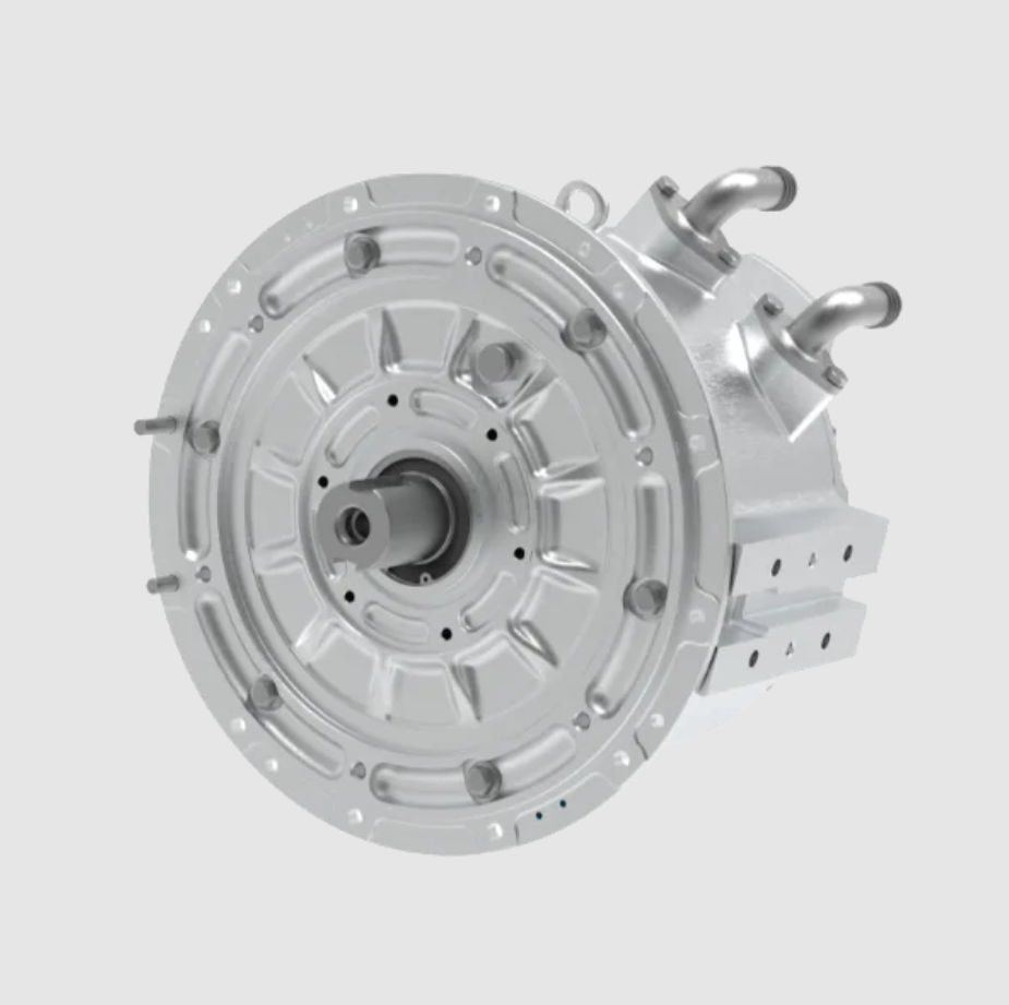
In my view, the most important engineering question is not whether sensorless control can work in a laboratory, but whether it can work reliably in an electric vehicle across cold starts, hot inverter conditions, low-speed crawling, high-speed field weakening, rough roads, electromagnetic interference, and parameter drift. I have found that a successful design must combine machine modeling, observer theory, signal processing, inverter nonlinearity compensation, parameter identification, and functional safety. I also believe that no single sensorless method dominates every operating region. Instead, a practical PMSM electric motor drive often uses a hybrid strategy: one method for zero-speed and low-speed operation, another for medium-speed and high-speed operation, and smooth transitions between them. This article explains the principles, mathematics, implementation choices, challenges, and solutions that I consider essential for applying sensorless control to the PMSM electric motor in electric vehicles.
PMSM Electric Motor Construction and Electric Vehicle Advantages
I first recall the physical structure of the PMSM electric motor. The stator is typically made of laminated silicon steel with three-phase windings distributed in slots. When three-phase currents flow through these windings, they create a rotating magnetomotive force and a rotating magnetic field. The rotor contains permanent magnets, often rare-earth magnets such as neodymium-iron-boron or samarium-cobalt, although ferrite-assisted or hybrid designs also exist for cost-sensitive applications. The interaction between the stator rotating field and the rotor permanent magnet field produces electromagnetic torque. If the rotor rotates at the same speed as the stator field, the machine operates synchronously. Because the rotor flux is provided by permanent magnets, the PMSM electric motor does not need rotor excitation current, which improves efficiency compared with induction machines in many operating regions.
I classify PMSM electric motors into two broad categories: surface-mounted permanent magnet machines and interior permanent magnet machines. In a surface-mounted PMSM electric motor, the magnets are mounted on the rotor surface, and the d-axis inductance is approximately equal to the q-axis inductance. In an interior permanent magnet PMSM electric motor, the magnets are buried inside the rotor, producing saliency, so the q-axis inductance is usually larger than the d-axis inductance. This saliency is useful because it produces reluctance torque and also enables high-frequency injection methods for sensorless control. In electric vehicle traction, interior permanent magnet machines are widely used because they can exploit both permanent magnet torque and reluctance torque, and they can operate in field weakening with better speed range capability.
| Machine Type | Rotor Excitation | Typical Efficiency | Power Density | Sensorless Suitability | Electric Vehicle Consideration |
|---|---|---|---|---|---|
| PMSM electric motor, surface-mounted | Permanent magnets | High | High | Moderate at low speed without saliency | Compact and efficient, but low-speed estimation can be difficult |
| PMSM electric motor, interior | Permanent magnets with saliency | Very high | Very high | Good when saliency is used | Excellent for traction, field weakening, and reluctance torque |
| Induction machine | Stator-induced rotor currents | Moderate to high | Moderate | Good with flux observers | Lower cost, but lower efficiency in some regions |
| Brushless DC machine | Permanent magnets | High | High | Good with back-EMF zero crossings | Simple control, but higher torque ripple |
| Wound-field synchronous machine | Rotor field winding | Moderate | Moderate | Possible with flux estimation | Controllable flux, but brushes and complexity |
From my perspective, the PMSM electric motor is particularly attractive for electric vehicles because of four properties. First, its high torque density allows a smaller and lighter machine for a given power requirement. Second, its high efficiency reduces battery drain and extends range. Third, its fast torque response supports traction control, regenerative braking, and stability functions. Fourth, its synchronous operation enables precise field-oriented control when rotor position is known. The challenge is that precise field-oriented control normally requires rotor position, and sensorless control must reconstruct that information accurately enough for torque control, efficiency optimization, and safety.
Dynamic Model of the PMSM Electric Motor
I use the dq reference frame model because it simplifies the PMSM electric motor equations and makes control design tractable. The first step is the Clarke transformation from three-phase quantities to stationary alpha-beta quantities. I write the current transformation as follows:
$$
\begin{bmatrix} i_\alpha \\ i_\beta \end{bmatrix}
=
\frac{2}{3}
\begin{bmatrix}
1 & -\frac{1}{2} & -\frac{1}{2} \\
0 & \frac{\sqrt{3}}{2} & -\frac{\sqrt{3}}{2}
\end{bmatrix}
\begin{bmatrix} i_a \\ i_b \\ i_c \end{bmatrix}
$$
The inverse Clarke transformation can be written as:
$$
\begin{bmatrix} i_a \\ i_b \\ i_c \end{bmatrix}
=
\begin{bmatrix}
1 & 0 \\
-\frac{1}{2} & \frac{\sqrt{3}}{2} \\
-\frac{1}{2} & -\frac{\sqrt{3}}{2}
\end{bmatrix}
\begin{bmatrix} i_\alpha \\ i_\beta \end{bmatrix}
$$
Next, I apply the Park transformation to rotate from the stationary frame to the rotor-oriented dq frame:
$$
\begin{bmatrix} i_d \\ i_q \end{bmatrix}
=
\begin{bmatrix}
\cos\theta_e & \sin\theta_e \\
-\sin\theta_e & \cos\theta_e
\end{bmatrix}
\begin{bmatrix} i_\alpha \\ i_\beta \end{bmatrix}
$$
Here, \(\theta_e\) is the electrical rotor angle. The inverse Park transformation is:
$$
\begin{bmatrix} i_\alpha \\ i_\beta \end{bmatrix}
=
\begin{bmatrix}
\cos\theta_e & -\sin\theta_e \\
\sin\theta_e & \cos\theta_e
\end{bmatrix}
\begin{bmatrix} i_d \\ i_q \end{bmatrix}
$$
For a PMSM electric motor, I express the stator voltage equations in the dq frame as:
$$
v_d = R_s i_d + L_d \frac{di_d}{dt} – \omega_e L_q i_q
$$
$$
v_q = R_s i_q + L_q \frac{di_q}{dt} + \omega_e L_d i_d + \omega_e \psi_f
$$
The stator flux linkages are:
$$
\lambda_d = L_d i_d + \psi_f
$$
$$
\lambda_q = L_q i_q
$$
The electromagnetic torque produced by the PMSM electric motor is:
$$
T_e = \frac{3}{2} p \left[ \psi_f i_q + (L_d – L_q) i_d i_q \right]
$$
For a surface-mounted PMSM electric motor, where \(L_d \approx L_q\), the torque expression simplifies to:
$$
T_e = \frac{3}{2} p \psi_f i_q
$$
The mechanical dynamics are governed by:
$$
J \frac{d\omega_m}{dt} = T_e – T_L – B \omega_m
$$
I relate mechanical speed and electrical speed through the pole pair number:
$$
\omega_e = p \omega_m
$$
I also use the electrical rotor angle derivative:
$$
\frac{d\theta_e}{dt} = \omega_e
$$
| Symbol | Meaning | Typical Unit | Role in Sensorless Control |
|---|---|---|---|
| \(v_d, v_q\) | Stator voltage in dq frame | V | Input to observer and current controller |
| \(i_d, i_q\) | Stator current in dq frame | A | Measured or estimated state |
| \(R_s\) | Stator resistance | \(\Omega\) | Changes with temperature and affects estimation |
| \(L_d, L_q\) | d-axis and q-axis inductance | H | Saliency enables injection methods |
| \(\psi_f\) | Permanent magnet flux linkage | Wb | Back-EMF magnitude and torque constant |
| \(\omega_e\) | Electrical angular speed | rad/s | Estimated by observer or PLL |
| \(\theta_e\) | Electrical rotor angle | rad | Required for Park transformation |
| \(p\) | Pole pair number | dimensionless | Relates mechanical and electrical speed |
| \(J\) | Rotor and load inertia | kg·m² | Affects speed dynamics |
| \(B\) | Viscous friction coefficient | N·m·s/rad | Mechanical damping |
I emphasize that the dq model is exact only when the rotor position is known. In sensorless control, the estimated angle \(\hat{\theta}_e\) replaces the true angle \(\theta_e\). If the angle error is \(\Delta\theta = \theta_e – \hat{\theta}_e\), then the estimated dq currents are rotated by that error. A small angle error can produce torque error and efficiency loss. A large angle error can cause loss of synchronism, overcurrent, or unstable torque production. Therefore, I treat angle estimation accuracy as a safety-relevant requirement for the PMSM electric motor drive.
Core Principle of Sensorless Control for the PMSM Electric Motor
I define sensorless control as the estimation of rotor position and speed without a mechanical shaft sensor. The estimation uses measurements that are already available in a typical inverter: phase currents, DC bus voltage, switching states, and sometimes temperature. The fundamental physical quantities that reveal rotor position are back electromotive force, magnetic saliency, and flux linkage. Back-EMF is proportional to speed and contains rotor angle information. Saliency creates inductance variation with rotor position, which can be detected by injecting a high-frequency voltage or current. Flux linkage can be estimated by integrating voltage minus resistive drop, although integration drift and parameter errors complicate this approach.
For a PMSM electric motor in the stationary alpha-beta frame, I write the back-EMF components as:
$$
e_\alpha = -\omega_e \psi_f \sin\theta_e
$$
$$
e_\beta = \omega_e \psi_f \cos\theta_e
$$
The stator current dynamics in the stationary frame can be expressed as:
$$
\frac{di_\alpha}{dt} = \frac{1}{L_s} \left( v_\alpha – R_s i_\alpha – e_\alpha \right)
$$
$$
\frac{di_\beta}{dt} = \frac{1}{L_s} \left( v_\beta – R_s i_\beta – e_\beta \right)
$$
If I can estimate \(e_\alpha\) and \(e_\beta\), then I can obtain the rotor angle from:
$$
\hat{\theta}_e = \operatorname{atan2} \left( -\hat{e}_\alpha, \hat{e}_\beta \right)
$$
I also estimate speed from the derivative of the angle or from a phase-locked loop. However, I have found that direct back-EMF estimation is difficult at low speed because the back-EMF magnitude is proportional to speed. At zero speed, the back-EMF is zero, so back-EMF-based methods cannot observe the rotor position without additional excitation or saliency exploitation. This limitation is one of the central challenges in sensorless control of the PMSM electric motor.
Common Sensorless Control Methods
I now review the methods that I consider most relevant to electric vehicle traction. Each method has a distinct operating region, computational burden, parameter sensitivity, and implementation complexity. In practice, I combine methods rather than relying on one alone.
Back-EMF and Flux Observer Methods
The back-EMF method estimates the induced voltage from the voltage equation and then extracts angle and speed. A simple implementation uses a Luenberger observer or a reduced-order observer. I can write the current observer as:
$$
\frac{d\hat{i}_\alpha}{dt} = \frac{1}{L_s} \left( v_\alpha – R_s \hat{i}_\alpha – \hat{e}_\alpha \right) + K_i \left( i_\alpha – \hat{i}_\alpha \right)
$$
$$
\frac{d\hat{i}_\beta}{dt} = \frac{1}{L_s} \left( v_\beta – R_s \hat{i}_\beta – \hat{e}_\beta \right) + K_i \left( i_\beta – \hat{i}_\beta \right)
$$
The estimated back-EMF is updated by an observer gain:
$$
\hat{e}_\alpha = K_e \left( i_\alpha – \hat{i}_\alpha \right)
$$
$$
\hat{e}_\beta = K_e \left( i_\beta – \hat{i}_\beta \right)
$$
I find this method intuitive and computationally light, but it is sensitive to stator resistance, inductance mismatch, and measurement noise. At low speed, the signal-to-noise ratio is poor. At high speed, discretization and inverter nonlinearity become more important. I therefore use it mainly in the medium-speed and high-speed regions, where back-EMF is strong.
Sliding Mode Observer
A sliding mode observer is a nonlinear observer that forces the estimation error onto a sliding surface. I define the current error as:
$$
s_\alpha = \hat{i}_\alpha – i_\alpha
$$
$$
s_\beta = \hat{i}_\beta – i_\beta
$$
The sliding surface vector is:
$$
s = \begin{bmatrix} s_\alpha \\ s_\beta \end{bmatrix}
$$
A common sliding mode control law uses the sign function:
$$
u_\alpha = k \operatorname{sign}(s_\alpha)
$$
$$
u_\beta = k \operatorname{sign}(s_\beta)
$$
The observer dynamics can be written as:
$$
\frac{d\hat{i}_\alpha}{dt} = \frac{1}{L_s} \left( v_\alpha – R_s \hat{i}_\alpha – u_\alpha \right)
$$
$$
\frac{d\hat{i}_\beta}{dt} = \frac{1}{L_s} \left( v_\beta – R_s \hat{i}_\beta – u_\beta \right)
$$
After the sliding mode is reached, the equivalent control contains the back-EMF information. I then low-pass filter the switching signal to extract \(\hat{e}_\alpha\) and \(\hat{e}_\beta\). The main advantage is strong robustness to parameter variation and external disturbance. The main disadvantage is chattering, which can increase acoustic noise, current ripple, and estimation error. I mitigate chattering by using a saturation function, a sigmoid function, a super-twisting algorithm, or an adaptive gain.
| Method | Operating Range | Parameter Sensitivity | Computational Cost | Main Strength | Main Weakness |
|---|---|---|---|---|---|
| Back-EMF observer | Medium to high speed | Moderate to high | Low | Simple and intuitive | Fails at zero and low speed |
| Sliding mode observer | Low to high speed with tuning | Low to moderate | Moderate | Robust to disturbances | Chattering and filtering delay |
| Model reference adaptive system | Medium to high speed | Moderate | Moderate | Adaptive speed estimation | Requires accurate reference model |
| Extended Kalman filter | Wide range | Moderate | High | Noise handling and state estimation | Tuning and matrix computation |
| High-frequency injection | Zero and low speed | Low to moderate | Moderate to high | Works at standstill | Noise, loss, and saliency dependence |
| Saliency tracking | Zero and low speed | Moderate | Moderate | Uses magnetic saliency | Requires sufficient saliency |
| Intelligent estimation | Depending on training | Data dependent | High | Can model nonlinearities | Verification and safety concerns |
Model Reference Adaptive System
In a model reference adaptive system, I compare the output of a reference model with the output of an adjustable model. The reference model is usually based on the actual PMSM electric motor voltage equations, while the adjustable model depends on the estimated speed. The error between the two models drives an adaptation mechanism that updates the estimated speed. I can define a typical error signal as:
$$
\varepsilon = \hat{i}_\alpha i_\beta – i_\alpha \hat{i}_\beta
$$
The estimated speed is then obtained through a proportional-integral adaptation law:
$$
\hat{\omega}_e = K_p \varepsilon + K_i \int \varepsilon \, dt
$$
I appreciate the conceptual clarity of this method, but I also recognize its dependence on the reference model. If the stator resistance or inductance changes, the error signal can be biased, leading to steady-state speed error. I therefore combine it with online parameter identification or use a robust adaptation law.
Extended Kalman Filter
The extended Kalman filter treats rotor speed and position as states and handles measurement noise statistically. I define a state vector as:
$$
x = \begin{bmatrix} i_d & i_q & \omega_e & \theta_e \end{bmatrix}^T
$$
The measurement vector is typically:
$$
z = \begin{bmatrix} i_d & i_q \end{bmatrix}^T
$$
The nonlinear state equation is:
$$
\dot{x} = f(x, u) + w
$$
The measurement equation is:
$$
z = h(x) + v
$$
Here, \(w\) is process noise and \(v\) is measurement noise. The extended Kalman filter linearizes the system around the current estimate and propagates the covariance matrix. I have found that it performs well over a wide speed range and can reject noise effectively. However, it requires careful tuning of covariance matrices, and its computational load is higher than simple observers. For an electric vehicle controller, I must ensure that the execution time remains within the control period and that numerical stability is maintained.
High-Frequency Injection
At zero and low speed, I use high-frequency injection because back-EMF is unavailable. The idea is to inject a high-frequency voltage signal into the d-axis or q-axis and measure the current response. Because the d-axis and q-axis inductances differ in an interior PMSM electric motor, the high-frequency current response contains rotor position information. A common injection voltage is:
$$
v_{dh} = V_h \cos(\omega_h t)
$$
The resulting high-frequency current in the estimated frame can be approximated as:
$$
i_{qh} \propto \Delta L \sin(2\Delta\theta)
$$
where \(\Delta L = L_q – L_d\) and \(\Delta\theta\) is the angle error. I demodulate the high-frequency current to extract the angle error and drive it to zero with a phase-locked loop or observer. This method works at standstill, which is essential for electric vehicle launch. However, it produces additional losses, acoustic noise, and torque ripple. I must select the injection frequency, amplitude, and demodulation filter carefully to balance estimation bandwidth, noise, and efficiency.
Saliency Tracking and INFORM
Saliency tracking methods use the spatial variation of inductance. The INFORM method uses current derivatives under different voltage pulse patterns to estimate the rotor position. I can express the current derivative in a stator-fixed frame as:
$$
\frac{di_s}{dt} = L_s^{-1}(\theta_e) \left( v_s – R_s i_s – e_s \right)
$$
Because \(L_s^{-1}(\theta_e)\) depends on rotor angle, I can extract position information from current derivatives. This method can work at low speed, but it requires precise current derivative measurement and is sensitive to inverter nonlinearity and noise. I consider it useful as a supplementary method rather than a standalone solution for all operating conditions.
Intelligent and Data-Driven Methods
I also investigate intelligent estimation methods, including neural networks, fuzzy logic, and reinforcement learning. These methods can approximate nonlinear relationships between measured signals and rotor position. However, I remain cautious about using them as primary safety-critical estimators because they require extensive training data, validation, and verification. In my view, they are more suitable for compensation, tuning, fault detection, or performance optimization than for replacing a deterministic observer in a production PMSM electric motor drive. A hybrid approach that uses a physics-based observer with a learned compensation term is more defensible for electric vehicle applications.
Implementation Architecture for the PMSM Electric Motor Drive
I implement sensorless control inside a field-oriented control architecture. The inverter measures phase currents, transforms them to the dq frame using the estimated angle, regulates d-axis and q-axis currents, and converts voltage commands into switching signals through space vector pulse width modulation. The sensorless observer runs in parallel with the current control loop. The estimated speed is used for speed control and field weakening. The estimated angle is used for coordinate transformation and torque control.
I show the main control loops and typical bandwidths in the table below. These values are not universal, but they represent the design ranges I have found useful for traction PMSM electric motor drives.
| Control Loop | Typical Bandwidth | Primary Input | Primary Output | Sensorless Interaction |
|---|---|---|---|---|
| Current loop | 500 Hz to 2 kHz | Current error | Voltage command | Needs accurate angle for dq transformation |
| Speed loop | 20 Hz to 200 Hz | Speed error | Torque or q-axis current command | Uses estimated speed |
| Position observer | 100 Hz to 1 kHz | Voltage and current | Estimated angle and speed | Core sensorless function |
| High-frequency injection loop | 1 kHz to 5 kHz | High-frequency current | Low-speed angle error | Active at standstill and low speed |
| Parameter identification | 1 Hz to 100 Hz | Voltage, current, temperature | Updated resistance and flux | Reduces observer mismatch |
| Field weakening | 10 Hz to 100 Hz | DC bus voltage and speed | d-axis current command | Depends on estimated speed and flux |
I use a phase-locked loop to extract angle and speed from the estimated back-EMF or from the high-frequency error signal. A typical PLL error for back-EMF estimation is:
$$
\varepsilon = -\hat{e}_\alpha \cos\hat{\theta}_e – \hat{e}_\beta \sin\hat{\theta}_e
$$
The speed estimate is generated by a proportional-integral controller:
$$
\hat{\omega}_e = K_p \varepsilon + K_i \int \varepsilon \, dt
$$
The angle estimate is obtained by integration:
$$
\hat{\theta}_e = \int \hat{\omega}_e \, dt
$$
I also ensure that the estimated angle is wrapped or normalized to avoid numerical overflow. In a discrete implementation, I write:
$$
\hat{\theta}_e(k+1) = \hat{\theta}_e(k) + T_s \hat{\omega}_e(k)
$$
where \(T_s\) is the sampling period. I have learned that the PLL gains must be tuned together with the observer gains. If the PLL is too fast, it amplifies noise. If it is too slow, it introduces phase lag and reduces stability margin. I often use adaptive gains that vary with speed: lower gains at low speed for noise rejection, and higher gains at high speed for fast tracking.
Challenges in Electric Vehicle Applications
I now turn to the practical challenges that I consider most important when applying sensorless control to a PMSM electric motor in an electric vehicle. These challenges are not independent. They interact through temperature, speed, load, and inverter behavior. A solution that improves one area can degrade another, so I treat the design as a multi-objective optimization problem.
Low-Speed and Zero-Speed Performance
At low speed, back-EMF is small, and the observer signal-to-noise ratio is poor. At zero speed, back-EMF is zero. This makes standstill position estimation impossible with pure back-EMF methods. Electric vehicles require reliable starting on slopes, creeping in traffic, and smooth torque at near-zero speed. If the estimated angle is wrong at standstill, the PMSM electric motor can produce reverse torque, excessive current, or fail to launch. I address this with high-frequency injection, saliency tracking, or a short open-loop startup followed by a transition to a closed-loop observer. The transition must be smooth because an abrupt switch can cause torque shock and current spikes.
Motor Parameter Variation
The parameters of a PMSM electric motor change during operation. Stator resistance increases with temperature. Permanent magnet flux linkage decreases with temperature and can also change due to irreversible demagnetization under fault conditions. Inductance changes with current due to magnetic saturation. These variations cause observer model mismatch. For example, if the actual resistance is higher than the model resistance, the estimated back-EMF may have an offset, leading to angle error. If the permanent magnet flux linkage is lower than the model value, the torque constant estimate is wrong, and speed estimation may drift. I use online parameter identification, thermal models, and robust observers to reduce this problem.
Electromagnetic Interference and Noise
An electric vehicle traction inverter switches at high frequency and high voltage. The switching process generates broadband electromagnetic interference. Current sensors, voltage sensors, and analog-to-digital converters can pick up noise. This noise propagates into the observer and corrupts angle estimation. I use differential signal routing, shielded cables, common-mode chokes, proper grounding, and analog filtering. I also use digital filtering, synchronous sampling, and observer bandwidth limits. In my experience, electromagnetic compatibility is not an afterthought; it must be designed together with the control algorithm.
Inverter Nonlinearity and Dead Time
Inverter nonlinearity arises from dead time, switch voltage drops, and parasitic capacitance. Dead time prevents shoot-through but distorts the output voltage, especially at low current and low speed. The voltage error can be approximated as:
$$
\Delta v = -\frac{T_d}{T_s} V_{dc} \operatorname{sign}(i)
$$
where \(T_d\) is dead time, \(T_s\) is switching period, \(V_{dc}\) is DC bus voltage, and \(i\) is phase current. This error acts as a disturbance to the observer and can cause significant angle estimation error at low speed. I compensate by estimating the current direction, applying a voltage correction, or using a dead-time compensation table. I also use current polarity detection with hysteresis to avoid chattering near zero current.
Thermal Effects and Magnetic Saturation
Thermal effects change resistance and magnet flux. Magnetic saturation changes inductance, especially in interior permanent magnet machines. Both effects are nonlinear and operating-point dependent. I use look-up tables, online identification, and temperature measurements to adapt the observer model. For a PMSM electric motor in a vehicle, the inverter coolant temperature, stator winding temperature, and rotor magnet temperature may differ. Rotor magnet temperature is difficult to measure directly, so I often estimate it from a thermal model or from flux linkage identification.
Load Torque Disturbance and Road Dynamics
The load torque on an electric vehicle traction motor is not constant. It varies with road grade, vehicle mass, rolling resistance, aerodynamic drag, regenerative braking, and wheel slip. These disturbances affect speed estimation and can excite observer dynamics. I design the speed loop and observer to reject load disturbances without amplifying noise. I also coordinate with the vehicle controller so that traction control and anti-lock braking actions do not cause unstable sensorless operation.
DC Bus Voltage Fluctuation
The DC bus voltage varies with battery state of charge, inverter operating point, and regenerative braking. Voltage measurement errors directly affect the observer because voltage is an input to the PMSM electric motor model. I use fast and accurate DC bus voltage sampling, compensate for sensor gain and offset, and include voltage dynamics in the observer where necessary. In field weakening, voltage margin is limited, so estimation errors can cause loss of current control.
Computational Burden and Real-Time Constraints
Sensorless algorithms must execute within the inverter control period, often tens of microseconds. High-order observers, Kalman filters, and high-frequency demodulation can be computationally expensive. I optimize by using reduced-order models, fixed-point or single-precision arithmetic, and efficient trigonometric approximations. I also schedule high-frequency injection only when needed, because continuous injection reduces efficiency and increases acoustic noise.
| Challenge | Physical Cause | Effect on PMSM Electric Motor Control | Solution I Apply |
|---|---|---|---|
| Low-speed estimation | Small back-EMF | Poor angle accuracy, starting failure | High-frequency injection, saliency tracking, hybrid transition |
| Zero-speed standstill | No back-EMF | No position information without excitation | Signal injection or initial position detection |
| Parameter variation | Temperature, saturation, aging | Observer model mismatch and angle error | Online identification, thermal model, robust observer |
| Electromagnetic interference | Fast switching, high voltage, high current | Noisy measurements and estimation jitter | Filtering, shielding, synchronous sampling, EMC design |
| Dead-time distortion | Inverter switching protection | Low-speed voltage error and angle bias | Dead-time compensation and current polarity detection |
| Magnetic saturation | High current and rotor geometry | Inductance variation and saliency change | Look-up tables and adaptive observer gains |
| Load disturbance | Road grade, mass, wheel slip | Speed error and torque ripple | Disturbance observer and vehicle-level coordination |
| DC bus variation | Battery and inverter operation | Voltage model error | Accurate sensing and feedforward compensation |
| Computational limit | Fast control period | Observer delay and numerical issues | Reduced-order algorithms and scheduled execution |
Solutions and Design Strategies
I now describe the solutions that I have found most effective. I do not claim that any single solution is sufficient. Instead, I combine several layers of estimation, compensation, and robustness.
Hybrid Estimation Strategy
I use a hybrid strategy that selects the estimation method based on speed and operating condition. At standstill and very low speed, I use high-frequency injection or initial position detection. In the transition region, I blend the injected signal estimate with a back-EMF observer. At medium and high speed, I use a back-EMF observer, sliding mode observer, or extended Kalman filter. The blending can be written as:
$$
\hat{\theta}_e = \alpha \hat{\theta}_{HF} + (1 – \alpha) \hat{\theta}_{BEMF}
$$
where \(\alpha\) is a weighting factor that decreases as speed increases. I design \(\alpha\) to be continuous and rate-limited to avoid torque shock. I also use a speed hysteresis band to prevent rapid switching between methods. In my experience, the transition region is where many sensorless drives fail, so I test it extensively under load and temperature variation.
High-Frequency Injection Optimization
I optimize high-frequency injection by selecting the injection axis, frequency, and amplitude. For an interior PMSM electric motor, d-axis injection is common because the saliency produces a q-axis current response that contains the angle error. I use a band-pass filter to extract the high-frequency component and a low-pass filter to remove switching noise. The demodulation signal is multiplied by the carrier and then low-pass filtered. I also use random or variable frequency injection to spread the acoustic spectrum and reduce tonal noise. If the saliency is small, I increase the injection amplitude within thermal and loss limits.
Online Parameter Identification
I use recursive least squares or Kalman filter-based identification to update stator resistance, permanent magnet flux linkage, and sometimes inductance. A general recursive least squares update is:
$$
\hat{\theta}(k) = \hat{\theta}(k-1) + K(k) \left[ y(k) – \phi^T(k) \hat{\theta}(k-1) \right]
$$
where \(\hat{\theta}\) is the parameter vector, \(\phi\) is the regressor, and \(K\) is the gain. For resistance identification, I can use the d-axis voltage equation at low speed or DC injection. For flux linkage identification, I use the q-axis voltage equation and known speed. I must ensure that the identification is not corrupted by the same noise that affects the observer. I often use separate time scales: fast current control, medium-speed observer, and slow parameter adaptation.
Robust and Adaptive Observers
I use sliding mode observers with boundary layers, super-twisting algorithms, and adaptive gains to improve robustness. A super-twisting observer reduces chattering while preserving disturbance rejection. I can write a simplified super-twisting law as:
$$
u = k_1 |s|^{1/2} \operatorname{sign}(s) + k_2 \int \operatorname{sign}(s) \, dt
$$
I tune \(k_1\) and \(k_2\) to achieve finite-time convergence and low chattering. I also use adaptive observers that adjust gains based on speed and current level. At low speed, I reduce observer bandwidth to reject noise. At high speed, I increase bandwidth to reduce phase lag.
Dead-Time and Inverter Nonlinearity Compensation
I compensate inverter nonlinearity by estimating the voltage error from phase current polarity. A practical compensation voltage is:
$$
v_{comp} = \Delta v \operatorname{sign}(i)
$$
I add \(v_{comp}\) to the voltage command before modulation. Because current polarity is uncertain near zero, I use a hysteresis band and a smooth transition function. I also calibrate the compensation table as a function of current magnitude and DC bus voltage. This improves low-speed angle estimation and reduces current distortion.
Filtering and Signal Conditioning
I use anti-aliasing filters before analog-to-digital conversion and digital filters after conversion. For back-EMF estimation, I use a low-pass filter with a cutoff frequency high enough to preserve dynamic response but low enough to reject switching noise. The filter introduces phase delay, so I compensate the estimated angle by the filter phase at the estimated speed:
$$
\Delta\theta_{comp} = \omega_e \tau_f
$$
where \(\tau_f\) is the equivalent filter time constant. I also use notch filters to remove specific switching harmonics and synchronous sampling to align current measurements with PWM. In my view, filtering is not a cosmetic step; it directly determines observer stability and accuracy.
Initial Position Detection
Before starting the PMSM electric motor, I need to know the initial rotor position. I use voltage pulse injection and measure current response. Because inductance varies with rotor position, the current peak differs for different voltage vectors. I compare the current responses and identify the sector. For interior permanent magnet machines, I can also use magnetic saturation saliency to distinguish north and south poles. This initial detection must be fast and must not produce excessive torque or noise. I sometimes combine it with high-frequency injection to refine the angle before closed-loop launch.
Fault Detection and Functional Safety
I design sensorless control with fault detection because an estimator can fail silently. I monitor current error, voltage error, speed estimate plausibility, angle error residual, and temperature. If the observer residual exceeds a threshold, I reduce torque, enter a limp-home mode, or switch to a backup estimation method. In a safety-critical electric vehicle, I also consider what happens if the position estimate is wrong. I limit torque rate, monitor acceleration consistency, and coordinate with the vehicle controller. I do not rely on a single observer without cross-checking.
| Design Layer | Function | Key Inputs | Key Outputs | Benefit for PMSM Electric Motor |
|---|---|---|---|---|
| Signal acquisition | Measure currents, voltages, temperature | Sensors and ADC | Filtered digital signals | Clean data for estimation |
| Initial position detection | Identify standstill angle | Pulse voltages and current response | Initial angle estimate | Reliable launch |
| Low-speed injection | Estimate angle without back-EMF | High-frequency voltage and current | Low-speed angle error | Standstill and crawl capability |
| Back-EMF observer | Estimate angle at medium and high speed | Voltage, current, model parameters | Angle and speed | Efficient high-speed operation |
| Parameter identification | Update resistance and flux | Voltage, current, temperature | Adapted model parameters | Reduced model mismatch |
| Compensation | Correct inverter and filter effects | Current polarity, filter delay | Voltage and angle corrections | Improved low-speed accuracy |
| Safety supervisor | Detect estimation faults | Residuals and plausibility checks | Torque limiting or fallback | Functional safety |
Performance Metrics and Validation
I evaluate sensorless control performance with several metrics. The most important are position error, speed error, torque ripple, current distortion, efficiency, acoustic noise, and robustness to parameter variation. I define root mean square position error as:
$$
\text{RMSE}_\theta = \sqrt{\frac{1}{N} \sum_{k=1}^{N} \left( \theta_k – \hat{\theta}_k \right)^2 }
$$
I define root mean square speed error as:
$$
\text{RMSE}_\omega = \sqrt{\frac{1}{N} \sum_{k=1}^{N} \left( \omega_k – \hat{\omega}_k \right)^2 }
$$
I also measure torque ripple using the peak-to-peak torque divided by average torque:
$$
T_{ripple} = \frac{T_{max} – T_{min}}{T_{avg}} \times 100\%
$$
For efficiency, I use:
$$
\eta = \frac{P_{mech}}{P_{elec}} = \frac{T_e \omega_m}{v_d i_d + v_q i_q}
$$
I validate the PMSM electric motor drive across a matrix of operating conditions. The table below shows the test scenarios I consider essential.
| Test Scenario | Speed Region | Load Condition | Temperature Condition | Primary Risk |
|---|---|---|---|---|
| Standstill launch | Zero speed | High torque demand | Cold and hot | Wrong initial angle and reverse torque |
| Creep and crawl | Very low speed | Low to moderate | Hot inverter | Poor signal-to-noise ratio |
| Urban acceleration | Low to medium | Transient | Variable | Method transition shock |
| Highway cruise | Medium to high | Steady | Hot | Parameter drift and efficiency |
| Field weakening | High speed | Light to moderate | Hot | Voltage margin and angle error |
| Regenerative braking | Medium to high | Negative torque | Variable | Observer direction and stability |
| Slope start | Zero to low | High load | Cold | Rollback and torque accuracy |
| Wheel slip | Transient | Rapid load change | Variable | Speed estimation disturbance |
| Electromagnetic interference | All | All | All | Measurement corruption |
| Parameter mismatch | All | All | Hot and cold | Angle bias and instability |
I use both simulation and hardware-in-the-loop testing. In simulation, I model the PMSM electric motor, inverter, battery, vehicle load, and sensor noise. I use finite-element-derived inductance tables for saturation and torque. In hardware-in-the-loop testing, I connect the inverter controller to a real-time motor model and inject fault conditions. Finally, I validate on a dynamometer and in a vehicle. I have found that dyno testing reveals thermal and low-speed issues that simulation can miss, while vehicle testing reveals electromagnetic compatibility, acoustic, and drivability issues that are difficult to model.
Application Scenarios in Electric Vehicles
I see sensorless control for the PMSM electric motor being valuable in several electric vehicle applications. The main traction motor is the most demanding because it requires high torque at zero speed, wide speed range, high efficiency, and functional safety. Auxiliary drives such as electric compressors, pumps, and fans also use PMSM electric motors, and sensorless control reduces cost and wiring. In e-axle architectures, the motor, gearbox, and inverter are integrated, so removing the position sensor simplifies the mechanical package and improves reliability. In all-wheel-drive electric vehicles, multiple PMSM electric motors must be coordinated, and sensorless control reduces the number of harnesses and connectors. I also see potential in range extenders, hybrid transmissions, and electric power take-off units.
| Application | Speed Range | Torque Demand | Sensorless Priority | Key Requirement |
|---|---|---|---|---|
| Main traction PMSM electric motor | Zero to high | Very high at low speed | Very high | Standstill torque and safety |
| Electric compressor | Medium to high | Moderate | High | Cost and noise reduction |
| Electric pump | Low to medium | Low to moderate | High | Reliability and compactness |
| Cooling fan | Low to high | Low | Moderate | Efficiency and EMC |
| E-axle integrated drive | Zero to high | High | Very high | Integration and fault tolerance |
| All-wheel-drive unit | Zero to high | High | High | Coordination and cost |
From my perspective, the main traction PMSM electric motor is the most difficult because the consequences of estimation failure are severe. A compressor or fan can tolerate a temporary speed error and recover, but a traction motor must produce accurate torque at standstill on a slope without rolling backward. Therefore, I design the traction sensorless controller with more redundancy, more conservative limits, and more extensive validation than auxiliary drives.
Future Trends
I expect several trends to shape the future of sensorless control for the PMSM electric motor. First, wide-bandgap devices such as silicon carbide and gallium nitride will increase switching frequency and reduce losses, but they will also increase electromagnetic interference and require faster sampling and more sophisticated filtering. Second, more powerful microcontrollers and digital signal processors will enable advanced observers, online identification, and artificial intelligence at the edge. Third, digital twins and cloud-based analytics will allow continuous tuning and predictive maintenance. Fourth, functional safety standards will require sensorless estimators to be developed with rigorous verification, fault detection, and fallback modes. Fifth, multi-motor drives and integrated e-axles will require distributed estimation and coordination. I also expect greater use of hybrid methods that combine physics-based observers with data-driven compensation.
| Future Trend | Expected Impact | Opportunity | Challenge | Relevance to PMSM Electric Motor |
|---|---|---|---|---|
| Wide-bandgap inverters | Higher switching frequency | Lower loss and faster control | More EMI and faster sampling | Requires robust observer filtering |
| Advanced microcontrollers | More computation | Complex observers and identification | Software complexity | Enables hybrid sensorless control |
| Digital twins | Continuous model updating | Predictive maintenance and tuning | Data management and validation | Improves parameter adaptation |
| Functional safety | Formal fault handling | Higher reliability | Verification cost | Requires estimator supervision |
| Artificial intelligence | Nonlinear compensation | Adaptive performance | Certification and explainability | Can assist but not replace deterministic observers |
| Integrated e-axle | Compact packaging | Lower cost and weight | Thermal and EMC coupling | Sensorless control simplifies integration |
My Design Recommendations
I conclude with the design recommendations that I apply when developing sensorless control for a PMSM electric motor in an electric vehicle. First, I model the machine accurately, including saturation, temperature, and inverter nonlinearity. Second, I use a hybrid estimator that covers zero speed through high speed. Third, I identify parameters online and adapt observer gains with operating conditions. Fourth, I compensate dead time, filter delay, and voltage measurement errors. Fifth, I validate across a wide matrix of temperatures, loads, speeds, and fault conditions. Sixth, I include fault detection and fallback strategies. Seventh, I optimize for acoustic noise and efficiency, not just angle accuracy. Eighth, I keep the algorithm implementable in real time with deterministic timing. Ninth, I coordinate sensorless control with vehicle-level torque management. Tenth, I document the assumptions and limits of each estimation method so that safety and calibration teams can verify them.
In my assessment, the PMSM electric motor will remain a dominant traction machine for electric vehicles because of its efficiency, power density, and controllability. Sensorless control will continue to mature as processors become faster, models become more accurate, and validation methods become more rigorous. The greatest value comes not from eliminating the position sensor alone, but from creating a drive that is more reliable, more compact, more efficient, and more capable across the full operating range. I believe that a well-designed sensorless PMSM electric motor drive can achieve performance close to a sensored drive while reducing cost and improving robustness. The key is to treat estimation as a system-level problem that includes the machine, inverter, sensors, software, thermal behavior, and vehicle dynamics. When I do that, the PMSM electric motor becomes not only a powerful traction source but also a resilient and intelligent component of the electric vehicle.
I also emphasize that sensorless control is not a single algorithm but a hierarchy of algorithms. The low-speed estimator, high-speed estimator, parameter identifier, compensation block, and safety supervisor must work together. If one block is poorly tuned, the entire PMSM electric motor drive can lose performance. Therefore, I tune the system iteratively: first the current loop, then the observer, then the speed loop, then the parameter adaptation, and finally the fault detection. I verify each step with step responses, frequency responses, and thermal soak tests. I also check the transition between estimation methods with slow ramps and fast transients. In my experience, this disciplined approach prevents many hidden failure modes.
Finally, I consider the economic and environmental impact. A sensorless PMSM electric motor drive reduces components, wiring, and assembly cost. It also improves reliability because there is no position sensor to fail in a harsh environment. Higher efficiency extends driving range and reduces energy consumption. Lower acoustic noise improves passenger comfort. These benefits support the broader goal of sustainable transportation. I therefore see sensorless control as an enabling technology for the next generation of electric vehicles, and I expect it to become increasingly standard in both main traction and auxiliary PMSM electric motor applications.