
I have been working on the control of traction machines for electric vehicles for a number of years, and in my experience the permanent-magnet synchronous machine has become the dominant choice for the main drive because of its high power density, high torque density, high efficiency, and compact rotor construction. In this article I present a complete design and analysis workflow for a PMSM electric motor drive that operates over a very wide speed range. I begin with the system context of an electric vehicle, then derive the mathematical model of the PMSM electric motor in the synchronous rotating reference frame, then develop the field-weakening control strategy that extends the operating range above the base speed, and finally I validate the whole scheme through simulation. I use the first person throughout because the design choices, the reasoning, and the conclusions are my own, and I want the reader to follow the same path that I followed when I built the controller.
1. Introduction
The electric vehicle industry has developed rapidly, and the traction motor has become the central component that determines acceleration performance, top speed, gradeability, and driving range. Among the candidate machine types, the PMSM electric motor stands out because it produces a high torque per unit volume, it achieves a high efficiency over a broad operating region, and it can be controlled with a relatively simple inverter. For these reasons I treat the PMSM electric motor as the reference traction machine in all of the analysis that follows.
An electric vehicle does not operate at a single speed or a single load. In real traffic it must start and stop frequently, climb slopes at low speed, cruise at moderate speed, and accelerate hard to overtake at high speed. Each of these conditions imposes a different requirement on the PMSM electric motor and on its controller. The low-speed conditions demand a large torque, which means a large stator current. The high-speed conditions demand a large rotational speed, which means a large back electromotive force, and that back electromotive force quickly approaches the available inverter voltage. When the back electromotive force equals the maximum inverter voltage, the PMSM electric motor reaches its base speed and it cannot be accelerated further with the conventional control law. To go beyond that point I must deliberately weaken the rotor flux, and this is exactly what field-weakening control does.
The classical field-weakening methods that I have studied and tested include the formula method, the look-up table method, the gradient method, and the negative d-axis current compensation method. Each of them has merit, but each of them also has a drawback. The formula method depends heavily on accurate machine parameters, and those parameters vary with temperature and with magnetic saturation. The look-up table method requires extensive calibration and it is sensitive to part-to-part variation. The gradient method can become unstable in the deep field-weakening region. The negative d-axis current compensation method can produce a torque ripple when the operating point crosses from one region to another. To overcome these limitations I propose a leading-angle field-weakening control strategy that regulates the phase of the stator current vector directly. This strategy keeps the PMSM electric motor within its safe operating envelope, it makes the transition from constant-torque operation to constant-power operation smooth, and it remains stable even in the deep field-weakening region.
The remainder of the article is organized as follows. I describe the electric vehicle system in Section 2. I derive the mathematical model of the PMSM electric motor in Section 3. I present the vector control law that I use below the base speed in Section 4. I develop the field-weakening principle and the voltage and current limits in Section 5. I define the three operating regions in Section 6. I formulate the leading-angle field-weakening strategy in Section 7. I describe the complete control structure in Section 8. I report the simulation results in Section 9. I state my conclusions in Section 10.
2. The PMSM Electric Motor in the Electric Vehicle System
From a system point of view, I divide the electric vehicle into three subsystems: the electric drive system, the power supply system, and the auxiliary system. The power supply system contains the traction battery, the battery management unit, and the on-board charger. Its role is to provide a stable dc bus for the PMSM electric motor, to monitor the state of charge and the state of health of the battery, and to manage the charging process. The auxiliary system improves handling, stability, and passenger comfort. The electric drive system is the heart of the vehicle, and its main components are the PMSM electric motor, the motor controller, the power electronic converter, and the transmission.
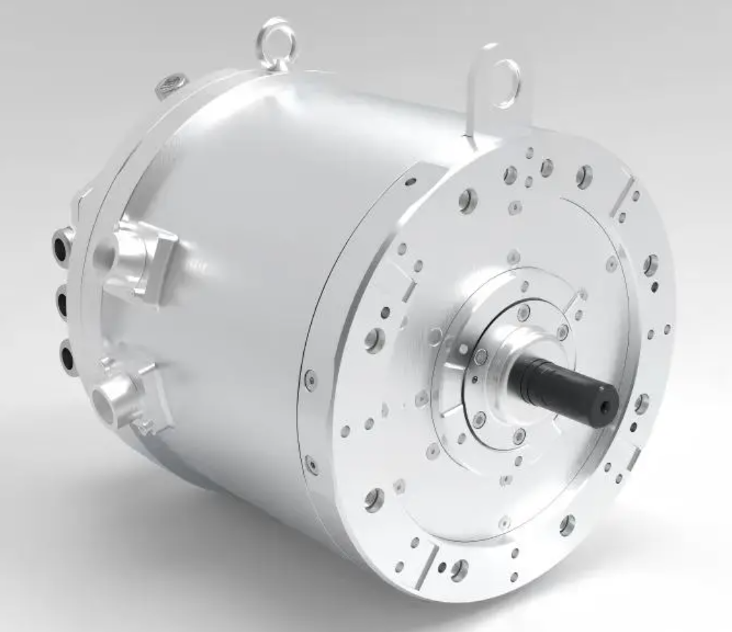
The working principle of the electric drive system is as follows. The vehicle control unit reads the accelerator pedal, the brake pedal, and the steering angle, and from these signals it interprets the intention of the driver. It then sends a target command to the motor controller. The motor controller generates the pulse-width modulation signals that switch the inverter, and the inverter applies the required voltage to the stator windings of the PMSM electric motor. The PMSM electric motor produces torque, the transmission delivers that torque to the wheels, and the vehicle moves.
In most driving conditions the electric vehicle operates in torque-control mode, in which the driver command is interpreted as a torque request. In a few special conditions, such as adaptive cruise control, the vehicle operates in speed-control mode, in which the driver command is interpreted as a speed request. To satisfy both requirements and to guarantee a good driving experience, I adopt a speed-and-current double closed-loop structure for the drive system. The outer loop regulates the speed of the PMSM electric motor, and the inner loops regulate the d-axis and q-axis currents. This structure gives me both accuracy in steady state and fast response in transients.
| Subsystem | Key components | Primary function |
|---|---|---|
| Electric drive system | PMSM electric motor, motor controller, power electronic converter, transmission | Convert electrical energy into mechanical torque and deliver it to the wheels |
| Power supply system | Traction battery, battery management unit, on-board charger | Supply a stable dc bus and manage charging and discharging |
| Auxiliary system | Steering, braking, thermal management, comfort devices | Improve handling, stability, comfort, and safety |
3. Mathematical Model of the PMSM Electric Motor
To design the controller I need a model that is accurate enough for control synthesis but simple enough for real-time implementation. I therefore make the following standard assumptions. I neglect magnetic saturation of the magnetic circuit. I neglect eddy-current and hysteresis losses. I neglect slotting effects and armature reaction effects. Under these assumptions I establish the model of the PMSM electric motor in the synchronous rotating d-q reference frame, where the d-axis is aligned with the rotor flux produced by the permanent magnets and the q-axis is displaced by ninety electrical degrees.
The voltage equations of the PMSM electric motor are
$$u_d = R_s i_d + L_d \frac{di_d}{dt} – \omega_e L_q i_q \tag{1}$$
$$u_q = R_s i_q + L_q \frac{di_q}{dt} + \omega_e \left( L_d i_d + \psi_f \right) \tag{2}$$
where \(u_d\) and \(u_q\) are the d-axis and q-axis stator voltages, \(i_d\) and \(i_q\) are the d-axis and q-axis stator currents, \(R_s\) is the stator resistance, \(L_d\) and \(L_q\) are the d-axis and q-axis inductances, \(\omega_e\) is the electrical angular speed, and \(\psi_f\) is the permanent-magnet flux linkage of the PMSM electric motor.
The flux equations are
$$\psi_d = L_d i_d + \psi_f \tag{3}$$
$$\psi_q = L_q i_q \tag{4}$$
The electromagnetic torque equation is
$$T_e = \frac{3}{2} n_p \left[ \psi_f i_q + \left( L_d – L_q \right) i_d i_q \right] \tag{5}$$
where \(n_p\) is the number of pole pairs of the PMSM electric motor. For a surface-mounted machine, in which the d-axis and q-axis inductances are equal, the reluctance term vanishes and the torque becomes proportional to the q-axis current alone:
$$T_e = \frac{3}{2} n_p \psi_f i_q \tag{6}$$
The mechanical motion equation is
$$T_e – T_L = J \frac{d\omega_r}{dt} + B \omega_r \tag{7}$$
where \(T_L\) is the load torque, \(J\) is the moment of inertia, \(B\) is the viscous friction coefficient, and \(\omega_r\) is the mechanical angular speed, which is related to the electrical angular speed by
$$\omega_e = n_p \omega_r \tag{8}$$
Substituting the flux equations into the voltage equations and the torque equation into the motion equation gives the complete model of the PMSM electric motor:
$$L_d \frac{di_d}{dt} = u_d – R_s i_d + \omega_e L_q i_q \tag{9}$$
$$L_q \frac{di_q}{dt} = u_q – R_s i_q – \omega_e L_d i_d – \omega_e \psi_f \tag{10}$$
$$J \frac{d\omega_r}{dt} = \frac{3}{2} n_p \left[ \psi_f i_q + \left( L_d – L_q \right) i_d i_q \right] – T_L – B \omega_r \tag{11}$$
Equations (9) and (10) show clearly that the d-axis and q-axis dynamics of the PMSM electric motor are coupled. The coupling term \(\omega_e L_q i_q\) appears in the d-axis equation, and the coupling terms \(\omega_e L_d i_d\) and \(\omega_e \psi_f\) appear in the q-axis equation. As the speed increases, the magnitude of these coupling terms increases, and the nonlinearity of the PMSM electric motor becomes more pronounced. This is one of the reasons why I include a decoupling block in the current loops of my controller.
| Symbol | Quantity | Unit |
|---|---|---|
| \(u_d, u_q\) | d-axis and q-axis stator voltages | V |
| \(i_d, i_q\) | d-axis and q-axis stator currents | A |
| \(R_s\) | Stator resistance | \(\Omega\) |
| \(L_d, L_q\) | d-axis and q-axis inductances | H |
| \(\psi_f\) | Permanent-magnet flux linkage | Wb |
| \(\psi_d, \psi_q\) | d-axis and q-axis flux linkages | Wb |
| \(\omega_r, \omega_e\) | Mechanical and electrical angular speeds | rad/s |
| \(n_p\) | Number of pole pairs | — |
| \(T_e, T_L\) | Electromagnetic torque and load torque | N·m |
| \(J\) | Moment of inertia | kg·m² |
| \(B\) | Viscous friction coefficient | N·m·s/rad |
| \(u_{smax}\) | Maximum stator phase voltage | V |
| \(i_{smax}\) | Maximum stator phase current | A |
4. Vector Control of the PMSM Electric Motor Below Base Speed
Below the base speed I want the PMSM electric motor to deliver the largest possible torque for a given stator current, because this minimizes the copper loss and therefore maximizes the efficiency and the driving range. For a surface-mounted PMSM electric motor, in which the d-axis and q-axis inductances are equal, the torque is proportional to the q-axis current, and the optimal strategy is to set the d-axis current to zero. I therefore adopt the \(i_d = 0\) vector control strategy in the low-speed region. This strategy satisfies the low-speed high-torque requirement and it improves the driving range of the electric vehicle.
When \(i_d = 0\), the torque equation of the PMSM electric motor reduces to
$$T_e = \frac{3}{2} n_p \psi_f i_q \tag{12}$$
and the stator current magnitude equals the q-axis current:
$$i_s = \sqrt{i_d^2 + i_q^2} = i_q \tag{13}$$
This means that the entire stator current is used to produce torque, and no current is wasted on flux weakening. The copper loss is then
$$P_{cu} = \frac{3}{2} R_s i_s^2 = \frac{3}{2} R_s i_q^2 \tag{14}$$
which is the minimum possible loss for a given torque. This is why the \(i_d = 0\) strategy is so attractive in the constant-torque region.
An alternative in the low-speed region is maximum torque per ampere control, which for an interior permanent-magnet machine with saliency exploits the reluctance torque. The MTPA condition is obtained by minimizing the current magnitude subject to a given torque, and it yields
$$i_d = \frac{\psi_f}{2 \left( L_q – L_d \right)} – \sqrt{\frac{\psi_f^2}{4 \left( L_q – L_d \right)^2} + i_q^2} \tag{15}$$
For a surface-mounted PMSM electric motor the inductances are equal, so the saliency term in the denominator goes to infinity and the MTPA condition degenerates to \(i_d = 0\). In this article I focus on the surface-mounted PMSM electric motor, so I use the \(i_d = 0\) strategy below the base speed.
| Speed region | Control strategy | d-axis current | Objective |
|---|---|---|---|
| Below base speed | \(i_d = 0\) vector control | Zero | Maximum torque per ampere, minimum copper loss |
| Below base speed with saliency | MTPA control | Negative | Exploit reluctance torque, reduce current magnitude |
| Above base speed | Field-weakening control | Negative | Reduce back electromotive force, extend speed range |
| Very high speed | MTPV control | Strongly negative | Maximum torque per volt, follow voltage limit |
5. Field-Weakening Principle for the PMSM Electric Motor
An inverter has a finite power rating, so the voltage and current that it can apply to the PMSM electric motor are limited. These two limits define the feasible operating region of the machine, and the controller must keep the operating point inside that region at all times. I now derive both limits and show how they lead naturally to the field-weakening requirement.
Let \(u_{smax}\) be the maximum available stator phase voltage. The voltage constraint is
$$u_d^2 + u_q^2 \leq u_{smax}^2 \tag{16}$$
If I neglect the stator resistance and the transient inductance terms in the steady state, the voltage equations of the PMSM electric motor become
$$u_d \approx -\omega_e L_q i_q \tag{17}$$
$$u_q \approx \omega_e \left( L_d i_d + \psi_f \right) \tag{18}$$
Substituting these approximations into the voltage constraint gives the voltage limit ellipse:
$$\left( L_d i_d + \psi_f \right)^2 + \left( L_q i_q \right)^2 \leq \left( \frac{u_{smax}}{\omega_e} \right)^2 \tag{19}$$
For a surface-mounted PMSM electric motor with \(L_d = L_q = L\), the ellipse becomes a circle centered at \(\left( -\psi_f / L, 0 \right)\) with radius \(u_{smax} / \left( L \omega_e \right)\):
$$\left( i_d + \frac{\psi_f}{L} \right)^2 + i_q^2 \leq \left( \frac{u_{smax}}{L \omega_e} \right)^2 \tag{20}$$
The radius of this voltage limit circle decreases as the electrical angular speed \(\omega_e\) increases. At low speed the circle is large and it does not restrict the operation of the PMSM electric motor. At high speed the circle becomes small, and the operating point must move along the circle rather than into the interior of the current limit circle.
Let \(i_{smax}\) be the maximum available stator phase current. The current constraint is
$$i_d^2 + i_q^2 \leq i_{smax}^2 \tag{21}$$
which is a circle centered at the origin with radius \(i_{smax}\). The PMSM electric motor can only operate in the intersection of the voltage limit circle and the current limit circle. When the speed rises above the base speed, the voltage limit circle shrinks until it no longer contains the point \(\left( 0, i_{smax} \right)\), which is the operating point of the \(i_d = 0\) strategy at full torque. At that moment the \(i_d = 0\) strategy becomes infeasible, and I must reduce the flux linkage seen by the stator. Because the rotor flux is produced by permanent magnets and cannot be changed directly, I produce a negative d-axis current that opposes the rotor flux. This is the essence of field weakening for the PMSM electric motor.
The effect of the negative d-axis current can be seen directly in the voltage limit circle. A negative \(i_d\) moves the operating point to the left along the d-axis, toward the center of the circle at \(-\psi_f / L\). The distance from the operating point to the center decreases, so the q-axis current that can be supported at a given speed increases. In this way the negative d-axis current extends the speed range of the PMSM electric motor at the cost of additional copper loss and a reduction in torque per ampere.
| Constraint | Mathematical form | Geometric shape | Effect of increasing speed |
|---|---|---|---|
| Voltage limit | \(\left( L_d i_d + \psi_f \right)^2 + \left( L_q i_q \right)^2 \leq \left( u_{smax} / \omega_e \right)^2\) | Ellipse, or circle for \(L_d = L_q\) | Radius shrinks as \(1 / \omega_e\) |
| Current limit | \(i_d^2 + i_q^2 \leq i_{smax}^2\) | Circle centered at the origin | Unchanged with speed |
| Feasible region | Intersection of the two limits | Lens-shaped region | Shrinks and shifts to the left |
6. Operating Regions of the PMSM Electric Motor
I divide the operating range of the PMSM electric motor into three regions according to the speed and according to which constraint is active. This division is useful because each region calls for a different current reference, and the transitions between the regions must be smooth.
Let \(\omega_b\) be the base speed of the PMSM electric motor, and let \(\omega_{mtpv}\) be the speed at which the voltage limit circle touches the maximum torque per volt curve. The three regions are defined as follows.
Region I: constant-torque operation. When the speed is at or below the base speed, \(\omega \leq \omega_b\), the voltage limit circle is large enough to contain the entire current limit circle, so the voltage constraint is inactive. The PMSM electric motor operates in the constant-torque region, and I use the \(i_d = 0\) strategy or the MTPA strategy to produce the maximum torque for the available current. The stator current trajectory follows the segment from the origin to point A, where point A lies on the current limit circle and corresponds to the maximum torque point.
Region II: constant-power operation. When the speed is between the base speed and the MTPV critical speed, \(\omega_b \leq \omega \leq \omega_{mtpv}\), the voltage limit circle has shrunk enough to cut into the current limit circle, so both constraints are active. The stator current trajectory follows the current limit circle from point A to point B. Point B is the intersection of the voltage limit circle and the maximum torque per volt curve, and it is the transition point between Region II and Region III. In this region the torque of the PMSM electric motor decreases as the speed rises, so the product of torque and speed, which is the power, remains approximately constant.
Region III: maximum torque per volt operation. When the speed is above the MTPV critical speed, \(\omega_{mtpv} \leq \omega \leq \omega_{max}\), the voltage limit circle has become so small that the current limit circle is no longer the active constraint. The stator current trajectory follows the maximum torque per volt curve from point B to point C. In this region the current magnitude is below \(i_{smax}\), and the operating point is determined entirely by the voltage limit. Region III exists only if the characteristic current \(\psi_f / L\) is smaller than the maximum stator current \(i_{smax}\).
The maximum torque per volt curve is obtained by maximizing the torque subject to the voltage constraint. For a surface-mounted PMSM electric motor the solution is
$$i_d = -\frac{\psi_f}{L} \tag{22}$$
which is the center of the voltage limit circle, and the corresponding q-axis current is
$$i_q = \frac{u_{smax}}{L \omega_e} \tag{23}$$
The torque then becomes
$$T_e = \frac{3}{2} n_p \psi_f i_q \tag{24}$$
and it decreases inversely with speed. This is the natural behaviour of the PMSM electric motor in the deep field-weakening region.
| Region | Speed range | Active constraint | Current trajectory | Torque behaviour |
|---|---|---|---|---|
| Region I | \(\omega \leq \omega_b\) | Current limit | Origin to point A | Constant maximum torque |
| Region II | \(\omega_b \leq \omega \leq \omega_{mtpv}\) | Current and voltage limits | Point A to point B | Torque decreases, power constant |
| Region III | \(\omega_{mtpv} \leq \omega \leq \omega_{max}\) | Voltage limit | Point B to point C | Torque decreases as \(1 / \omega\) |
7. Leading-Angle Field-Weakening Control Strategy
The central contribution of my work is the leading-angle field-weakening control strategy. Instead of computing the d-axis and q-axis current references from a parameter-dependent formula or from a large look-up table, I regulate the phase angle of the stator current vector directly. I call this angle the leading angle and I denote it by \(\gamma\). The d-axis and q-axis current references are then
$$i_d = i_s \sin \gamma \tag{25}$$
$$i_q = i_s \cos \gamma \tag{26}$$
where \(i_s\) is the magnitude of the stator current vector. When the speed is below the base speed, the leading angle is zero, so \(i_d = 0\) and \(i_q = i_s\). The PMSM electric motor operates in the constant-torque region with the \(i_d = 0\) strategy. When the speed rises above the base speed, the leading angle becomes negative, so \(i_d = i_s \sin \gamma < 0\) and the d-axis current opposes the rotor flux. The PMSM electric motor then operates in the constant-power region and the field weakening takes effect.
The leading angle is adjusted by a voltage feedback loop. The inverter dc bus voltage and the pulse-width modulation scheme determine the maximum stator voltage vector, and therefore they determine the maximum d-axis demagnetizing current that can be produced. I measure the stator voltage vector magnitude and compare it with the maximum value that the inverter can deliver. The error drives a proportional-integral controller whose output is the leading angle. When the measured voltage is below the limit, the controller saturates in the positive direction and the leading angle remains at zero. When the measured voltage reaches the limit, the controller comes out of saturation and the leading angle becomes negative. The stronger the voltage error, the more negative the leading angle, and the larger the demagnetizing current.
With space-vector pulse-width modulation, the maximum undistorted sinusoidal phase voltage that the inverter can produce is
$$u_{smax} = \frac{U_{dc}}{\sqrt{3}} \tag{27}$$
where \(U_{dc}\) is the dc bus voltage. This is the threshold that I use in the voltage feedback loop. The complete field-weakening law can be summarized as
$$\gamma = \begin{cases} 0, & u_s \leq u_{smax} \\ K_p \left( u_s – u_{smax} \right) + K_i \int \left( u_s – u_{smax} \right) dt, & u_s > u_{smax} \end{cases} \tag{28}$$
subject to the constraint
$$-\frac{\pi}{2} \leq \gamma < 0 \tag{29}$$
The lower bound \(-\pi / 2\) corresponds to a purely demagnetizing current, in which the entire stator current is aligned with the negative d-axis and no torque is produced. In practice the controller never reaches this bound because the voltage limit circle always leaves some room for q-axis current, but the bound is useful as a theoretical limit.
The advantages of the leading-angle strategy are as follows. First, it does not require an accurate value of the permanent-magnet flux linkage or of the inductances, because the voltage feedback loop corrects the operating point automatically. Second, it produces a smooth transition between the constant-torque region and the constant-power region, because the leading angle changes continuously from zero to a negative value. Third, it remains stable in the deep field-weakening region, because the voltage feedback loop continues to regulate the operating point even when the voltage limit circle is very small. Fourth, it is simple to implement, because it requires only one additional proportional-integral controller and a voltage magnitude calculation.
| Method | Parameter dependence | Stability in deep field weakening | Transition smoothness | Implementation complexity |
|---|---|---|---|---|
| Formula method | High | Moderate | Moderate | Low |
| Look-up table method | Medium | Good | Moderate | High |
| Gradient method | Medium | Poor | Moderate | Medium |
| Negative d-axis compensation | High | Moderate | Poor | Low |
| Leading-angle method | Low | Good | Good | Medium |
8. Control Structure of the PMSM Electric Motor Drive
The control structure that I use is a multi-loop system. It contains one speed loop, one voltage loop, and two current loops. The speed loop is the outer loop and it regulates the mechanical speed of the PMSM electric motor. The voltage loop is the field-weakening loop and it regulates the magnitude of the stator voltage vector. The two current loops are the innermost loops and they regulate the d-axis and q-axis currents.
The speed loop receives the speed reference from the vehicle control unit and the measured speed from the position sensor or from a sensorless estimator. The speed error is processed by a proportional-integral controller, and the output is the q-axis current reference \(i_q^*\). Because the q-axis current is proportional to the torque of the PMSM electric motor, this loop translates the speed demand into a torque demand. The speed loop therefore determines the accuracy of the speed regulation.
The current loops receive the d-axis and q-axis current references and the measured currents. Each loop uses a proportional-integral controller to generate the corresponding voltage reference. The current loops are responsible for the dynamic response of the drive. When the load torque changes suddenly, the current loops must react quickly to keep the actual currents close to their references and to prevent the speed of the PMSM electric motor from deviating significantly.
Because the d-axis and q-axis dynamics of the PMSM electric motor are coupled, as shown in equations (9) and (10), I add a decoupling block to the current loops. The decoupling terms are
$$u_{d,dec} = -\omega_e L_q i_q \tag{30}$$
$$u_{q,dec} = \omega_e L_d i_d + \omega_e \psi_f \tag{31}$$
These terms cancel the coupling in the plant, so the d-axis current loop and the q-axis current loop become independent. This allows me to tune the two loops separately and to achieve precise control of both the flux and the torque of the PMSM electric motor.
The voltage loop computes the magnitude of the stator voltage vector from the d-axis and q-axis voltage references:
$$u_s = \sqrt{u_d^{*2} + u_q^{*2}} \tag{32}$$
It then compares this magnitude with the maximum available voltage \(u_{smax}\) and produces the leading angle \(\gamma\) through a proportional-integral controller. The leading angle is used to compute the d-axis current reference:
$$i_d^* = i_s^* \sin \gamma \tag{33}$$
where \(i_s^*\) is the magnitude of the stator current reference. The q-axis current reference is
$$i_q^* = i_s^* \cos \gamma \tag{34}$$
In the constant-torque region, \(\gamma = 0\), so \(i_d^* = 0\) and \(i_q^* = i_s^*\). In the field-weakening region, \(\gamma < 0\), so \(i_d^* < 0\) and the d-axis current weakens the rotor flux. The transition between the two regions is automatic and continuous, because the leading angle changes continuously with the voltage error.
| Loop | Controlled variable | Reference | Controller output | Function |
|---|---|---|---|---|
| Speed loop | Mechanical speed \(\omega_r\) | \(\omega_r^*\) | \(i_q^*\) | Regulate speed with high accuracy |
| Current loop d-axis | d-axis current \(i_d\) | \(i_d^*\) | \(u_d^*\) | Regulate flux-weakening current |
| Current loop q-axis | q-axis current \(i_q\) | \(i_q^*\) | \(u_q^*\) | Regulate torque current |
| Voltage loop | Stator voltage magnitude \(u_s\) | \(u_{smax}\) | \(\gamma\) | Activate and regulate field weakening |
9. Simulation Verification
I built a simulation model of the complete electric vehicle drive with the PMSM electric motor and its controller in a standard simulation environment. I set the dc bus voltage to 800 V and I used space-vector pulse-width modulation with a switching frequency of 10 kHz. The initial speed reference was 8000 r/min and the load torque was 70 N·m. At \(t = 0.5\) s I increased the speed reference to 14000 r/min, and at \(t = 1.0\) s I increased it again to 18000 r/min. I recorded the speed, the stator voltage magnitude, the leading angle, and the d-axis current.
| Parameter | Value | Unit |
|---|---|---|
| DC bus voltage | 800 | V |
| Switching frequency | 10 | kHz |
| Initial speed reference | 8000 | r/min |
| Second speed reference | 14000 | r/min |
| Third speed reference | 18000 | r/min |
| Load torque | 70 | N·m |
| Speed step times | 0.5 and 1.0 | s |
The results confirm the expected behaviour. During the interval from 0 s to 0.5 s the PMSM electric motor runs below its base speed. The stator voltage magnitude stays below the limit \(U_{dc} / \sqrt{3}\), the leading angle stays at zero, and the d-axis current stays at zero. The machine operates in the constant-torque region with the \(i_d = 0\) strategy, and the torque is determined entirely by the q-axis current.
During the interval from 0.5 s to 1.0 s the speed of the PMSM electric motor exceeds the base speed. The stator voltage reaches the limit, and the voltage loop comes out of saturation. The leading angle becomes negative, the d-axis current becomes negative, and the rotor flux is weakened. The machine operates in the constant-power region. The negative d-axis current reduces the flux linkage seen by the stator, which reduces the back electromotive force and allows the PMSM electric motor to continue accelerating even though the voltage limit circle has shrunk.
During the interval from 1.0 s to 1.5 s the speed of the PMSM electric motor rises further. The stator voltage magnitude remains at its maximum value, and the voltage loop produces an even more negative leading angle. The d-axis current becomes more negative, and the field weakening becomes deeper. The PMSM electric motor remains stable throughout, and it reaches the final speed reference without oscillation.
These results show that the leading-angle field-weakening strategy achieves a fast response, good stability, and a smooth transition between the constant-torque and constant-power regions. The PMSM electric motor operates stably above its base speed for an extended period, and its speed range is significantly widened.
| Time interval | Speed condition | Leading angle | d-axis current | Operating region |
|---|---|---|---|---|
| 0–0.5 s | Below base speed | 0 rad | 0 A | Constant torque |
| 0.5–1.0 s | Above base speed | Negative | Negative | Constant power |
| 1.0–1.5 s | Deep field weakening | More negative | More negative | Maximum torque per volt |
10. Conclusion
I have presented a complete design and analysis of a field-weakening control strategy for a PMSM electric motor used in an electric vehicle. I began with the system context and showed how the electric drive system, the power supply system, and the auxiliary system interact. I then derived the mathematical model of the PMSM electric motor in the synchronous rotating reference frame and I identified the nonlinear coupling between the d-axis and q-axis dynamics. I explained why the conventional \(i_d = 0\) vector control strategy is optimal below the base speed and why it must be replaced by field-weakening control above the base speed. I derived the voltage limit ellipse and the current limit circle, and I used them to define the three operating regions of the PMSM electric motor. I then formulated the leading-angle field-weakening strategy, in which a voltage feedback loop adjusts the phase angle of the stator current vector so that the machine operates within its voltage and current limits at all speeds. I described the complete multi-loop control structure, including the speed loop, the two current loops with decoupling, and the voltage loop. Finally, I validated the strategy by simulation and I showed that the PMSM electric motor can operate stably over a very wide speed range with a smooth transition between operating regions.
From my perspective, the leading-angle strategy offers three practical benefits for the PMSM electric motor. First, it reduces the dependence on machine parameters, which is important because the permanent-magnet flux linkage and the inductances vary with temperature and with saturation. Second, it improves the stability of the deep field-weakening region, which is critical for high-speed cruising and for overtaking manoeuvres. Third, it produces a smooth transition between the constant-torque and constant-power regions, which improves the driving experience and reduces the mechanical stress on the drivetrain. I believe that these benefits make the leading-angle field-weakening strategy a strong candidate for the next generation of electric vehicle traction controllers based on the PMSM electric motor.
There are several directions that I intend to pursue in future work. One is the extension of the strategy to interior permanent-magnet machines, in which the saliency produces a reluctance torque that can be exploited together with the field weakening. Another is the integration of the field-weakening loop with a sensorless position estimator, so that the cost and the complexity of the drive can be reduced. A third is the adaptation of the controller gains to compensate for changes in the dc bus voltage and in the machine temperature. Each of these directions has the potential to further improve the performance of the PMSM electric motor in electric vehicle applications.
References
[1] Y. Zhang, T. Fan, P. Ning, et al., “High-performance field-weakening control strategy for vehicle permanent-magnet synchronous motors,” Journal of Power Supply, vol. 22, no. 2, pp. 378–385, 2024.
[2] F. Shen, “Research on field-weakening speed regulation system of permanent-magnet synchronous motor for electric vehicles,” M.S. thesis, Xiangtan University, 2020.
[3] Z. Gan, Y. Wang, D. Miao, et al., “Current vector control of permanent-magnet synchronous motor with wide speed range,” Journal of Electric Machines and Control, vol. 24, no. 1, pp. 1–9, 2020.