
In my analysis of high-speed drive systems, the PMSM electric motor occupies a central position because it combines high efficiency, high power density, and strong dynamic performance. I have organized this article around the operating mechanism, the control architecture, the key technical bottlenecks, and a composite vector control method that I consider suitable for high-speed PMSM electric motor applications. Throughout the discussion, I use mathematical models, comparison tables, and design equations to summarize the main relationships. My purpose is to show how a high-speed PMSM electric motor can be controlled with better speed tracking, lower torque ripple, reduced current harmonics, and stronger fault tolerance.
The PMSM electric motor is widely used in aerospace, robotics, electric vehicles, precision manufacturing, and energy conversion. When the PMSM electric motor operates at high speed, the electrical frequency becomes large, the iron loss and eddy-current loss increase, the switching frequency becomes limited relative to the fundamental frequency, and the mechanical stress on the rotor becomes significant. Therefore, the drive control of a high-speed PMSM electric motor cannot be treated as a simple extension of low-speed control. I need to consider the coupling between electromagnetic design, power electronics, thermal behavior, sensorless estimation, and fault diagnosis.
My Perspective on High-Speed PMSM Electric Motor Drive Systems
From my point of view, a high-speed PMSM electric motor drive system is a multi-domain system. It contains an inverter, a power converter, a drive stage, a controller, sensors or observers, and protection logic. The inverter transforms DC power into AC power with adjustable amplitude and frequency. The power converter manages energy flow under different voltage levels. The drive stage applies the switching signals to the PMSM electric motor. The controller regulates current, speed, torque, flux, and fault response. For a high-speed PMSM electric motor, the control bandwidth must be high enough to track the fundamental frequency while still suppressing switching harmonics.
I have found that vector control remains the most practical foundation for a high-speed PMSM electric motor. Vector control transforms the three-phase stationary frame into a rotor-oriented d-q frame, so that the PMSM electric motor behaves like a separately excited DC machine in terms of torque and flux control. The d-axis current controls flux, while the q-axis current controls torque. This decoupling is essential for a high-speed PMSM electric motor because the available voltage margin is small and the current dynamics are fast.
The general voltage equations for a PMSM electric motor in the d-q frame are:
$$v_d = R_s i_d + L_d \frac{di_d}{dt} – \omega_e L_q i_q$$
$$v_q = R_s i_q + L_q \frac{di_q}{dt} + \omega_e \left( L_d i_d + \psi_f \right)$$
In these equations, \(v_d\) and \(v_q\) are the stator voltage components, \(i_d\) and \(i_q\) are the stator current components, \(R_s\) is the stator resistance, \(L_d\) and \(L_q\) are the d-axis and q-axis inductances, \(\omega_e\) is the electrical angular speed, and \(\psi_f\) is the permanent magnet flux linkage. For a high-speed PMSM electric motor, the cross-coupling terms \(\omega_e L_q i_q\) and \(\omega_e L_d i_d\) become large. I must compensate them carefully; otherwise the current controller loses accuracy and the PMSM electric motor may enter an unstable region.
The electromagnetic torque of the PMSM electric motor is:
$$T_e = \frac{3}{2} p \left[ \psi_f i_q + \left( L_d – L_q \right) i_d i_q \right]$$
where \(p\) is the pole pair number. The mechanical equation is:
$$T_e – T_L = J \frac{d\omega_m}{dt} + B \omega_m$$
where \(T_L\) is the load torque, \(J\) is the inertia, \(B\) is the damping coefficient, and \(\omega_m\) is the mechanical angular speed. The electrical speed and mechanical speed are related by:
$$\omega_e = p \omega_m$$
For high-speed operation, the voltage limit is one of the most important constraints. The stator voltage magnitude must satisfy:
$$v_s = \sqrt{v_d^2 + v_q^2} \leq \frac{V_{dc}}{\sqrt{3}}$$
where \(V_{dc}\) is the DC bus voltage. This inequality explains why field weakening becomes necessary when the PMSM electric motor exceeds its base speed. I have observed that if the controller does not reduce the flux-producing current properly, the back electromotive force of the PMSM electric motor can exceed the inverter voltage capability, and the current regulator saturates.
I summarize the main high-speed constraints in the following table.
| Constraint | Physical Cause | Effect on PMSM Electric Motor | Control Response |
|---|---|---|---|
| Voltage limit | Finite DC bus and inverter modulation limit | Loss of current controllability at high speed | Field weakening and MTPA transition |
| Switching frequency limit | Power device loss and thermal limit | Low carrier ratio and increased harmonics | SVPWM, synchronous sampling, harmonic suppression |
| Iron and eddy-current loss | High electrical frequency and flux variation | Efficiency reduction and rotor heating | Loss-model-based current distribution |
| Rotor mechanical stress | Centrifugal force at high speed | Risk of magnet or sleeve failure | Mechanical derating and fault detection |
| Sensor limitations | Installation space and reliability | Increased weight and reduced robustness | Sensorless vector control |
| Electromagnetic interference | Fast switching and parasitic capacitance | Noise in current and voltage feedback | Filtering, shielding, and observer design |
I believe that the high-speed PMSM electric motor must be treated as a tightly coupled plant. A good current controller alone is not enough. The speed observer, the inverter nonlinearity compensation, the thermal protection, and the fault-tolerant strategy all influence the final performance of the PMSM electric motor.
Mathematical Model and Operating Mechanism of the PMSM Electric Motor
When I derive the model of a PMSM electric motor, I usually start from the stator voltage equations in the stationary reference frame and then apply the Park transformation. The result is the d-q model given above. For a surface-mounted PMSM electric motor, \(L_d \approx L_q\), so the reluctance torque term is small. For an interior PMSM electric motor, \(L_d < L_q\), and the reluctance torque can be used to improve efficiency. In high-speed applications, the interior PMSM electric motor is often preferred because the rotor structure provides mechanical robustness and additional torque capability.
The stator flux linkage components are:
$$\psi_d = L_d i_d + \psi_f$$
$$\psi_q = L_q i_q$$
The stator flux magnitude is:
$$\psi_s = \sqrt{\psi_d^2 + \psi_q^2}$$
The power factor and the current angle are important for the PMSM electric motor. If I define the current angle \(\beta\) with respect to the q-axis, then:
$$i_d = -i_s \sin \beta$$
$$i_q = i_s \cos \beta$$
The torque can then be written as:
$$T_e = \frac{3}{2} p \left[ \psi_f i_s \cos \beta + \frac{1}{2} \left( L_d – L_q \right) i_s^2 \sin 2\beta \right]$$
For maximum torque per ampere, I set the derivative of torque with respect to \(\beta\) to zero. For an interior PMSM electric motor with \(L_q > L_d\), the MTPA condition is approximately:
$$i_d = \frac{-\psi_f + \sqrt{\psi_f^2 + 8 \left( L_q – L_d \right)^2 i_q^2}}{4 \left( L_q – L_d \right)}$$
Alternatively, some formulations use:
$$i_d = \frac{-\psi_f + \sqrt{\psi_f^2 + 4 \left( L_q – L_d \right)^2 i_q^2}}{2 \left( L_q – L_d \right)}$$
I always verify the sign convention and the inductance difference before implementing MTPA in a high-speed PMSM electric motor. A small error in the MTPA angle can increase copper loss and reduce the voltage margin.
At high speed, the back electromotive force is:
$$e_q = \omega_e \psi_f$$
$$e_d = -\omega_e L_q i_q$$
The terminal voltage must overcome the back electromotive force, the resistive drop, and the inductive drop. Therefore, the available current loop bandwidth is reduced. I summarize the operating regions of a high-speed PMSM electric motor in the table below.
| Operating Region | Speed Condition | Current Strategy | Main Limitation |
|---|---|---|---|
| Low-speed constant-torque region | \(\omega_e \leq \omega_{base}\) | MTPA or \(i_d = 0\) | Current and thermal limit |
| Constant-power region | \(\omega_e > \omega_{base}\) | Field weakening with negative \(i_d\) | Voltage limit |
| Deep field-weakening region | Near maximum speed | Flux weakening and current angle optimization | Stability and parameter sensitivity |
| Fault-tolerant region | After fault detection | Current redistribution and torque derating | Inverter and winding limits |
I also note that the PMSM electric motor model contains parameters that vary with temperature and magnetic saturation. The stator resistance increases with temperature, while the permanent magnet flux decreases as temperature rises. These variations affect the observer and the current controller. For a high-speed PMSM electric motor, online parameter adaptation or robust control is therefore desirable.
Key Control Problems I Identify for the High-Speed PMSM Electric Motor
In my assessment, the high-speed PMSM electric motor drive has several key problems. First, the rotor position must be estimated accurately without a mechanical sensor, because sensor installation increases cost, weight, and failure probability. Second, the current loop must reject harmonics caused by inverter nonlinearity, dead time, and low carrier ratio. Third, the torque ripple must be suppressed to avoid mechanical vibration and acoustic noise. Fourth, the controller must remain stable during field weakening. Fifth, the drive must tolerate faults such as open-phase, short-circuit, and sensor failure. Sixth, the thermal limit of the PMSM electric motor and the inverter must be respected.
I have summarized these problems and the corresponding control objectives in the following table.
| Problem | Root Cause | Control Objective | Typical Method |
|---|---|---|---|
| Rotor position estimation | No mechanical sensor or sensor failure | Accurate speed and angle at high speed | Back-EMF observer, flux observer, Luenberger observer |
| Current harmonic distortion | Dead time, inverter nonlinearity, low carrier ratio | Low THD and smooth torque | Harmonic suppression, dead-time compensation |
| Torque ripple | Cogging torque, flux harmonics, current harmonics | Low ripple and low vibration | SVPWM, current shaping, observer-based compensation |
| Field-weakening stability | Voltage saturation and parameter variation | Stable operation above base speed | Voltage margin control, anti-windup, MTPA transition |
| Fault tolerance | Winding, inverter, or sensor fault | Continued operation with reduced torque | Four-leg inverter, redundant phases, fault diagnosis |
| Thermal protection | Copper loss, iron loss, switching loss | Limit temperature rise | Loss model, thermal observer, current derating |
I think the most difficult problem is the simultaneous requirement of high bandwidth and low harmonic distortion. A high-speed PMSM electric motor has a high fundamental frequency, so the ratio of switching frequency to fundamental frequency is low. If I increase the switching frequency to improve harmonic performance, the inverter loss increases. If I reduce the switching frequency to improve efficiency, the current ripple increases. Therefore, I need a control strategy that makes better use of the available switching vectors and the observer information.
Sensorless Vector Control for the PMSM Electric Motor
Sensorless vector control is one of the most active areas in high-speed PMSM electric motor research. I classify the methods into three families: back-EMF estimation, stator current observer, and flux observer. Each family has advantages and limitations. In a high-speed PMSM electric motor, back-EMF is large, so back-EMF-based estimation can be effective. However, at low speed, the back-EMF is small, and the signal-to-noise ratio is poor. A hybrid method is often used to cover the full speed range.
The back-EMF components in the stationary frame are:
$$e_\alpha = -\omega_e \psi_f \sin \theta_e$$
$$e_\beta = \omega_e \psi_f \cos \theta_e$$
From these components, the electrical angle can be estimated as:
$$\hat{\theta}_e = \tan^{-1} \left( \frac{-\hat{e}_\alpha}{\hat{e}_\beta} \right)$$
The speed can be obtained by differentiating the estimated angle or by using a phase-locked loop. A phase-locked loop for the PMSM electric motor can be written as:
$$\Delta \theta = \hat{\theta}_e – \theta_e^*$$
$$\hat{\omega}_e = k_p \Delta \theta + k_i \int \Delta \theta \, dt$$
$$\hat{\theta}_e = \int \hat{\omega}_e \, dt$$
For a stator current observer, I write the PMSM electric motor model as a state-space system:
$$\dot{x} = A x + B u$$
$$y = C x$$
where the state vector may include stator current and back-EMF. A Luenberger observer has the form:
$$\dot{\hat{x}} = A \hat{x} + B u + L \left( y – C \hat{x} \right)$$
where \(L\) is the observer gain matrix. The estimation error dynamics are:
$$\dot{e} = \left( A – L C \right) e$$
I choose \(L\) so that \(A – L C\) is stable and fast enough for the high-speed PMSM electric motor. A flux observer estimates the stator flux and then extracts the rotor angle. The stator flux in the stationary frame is:
$$\psi_\alpha = \int \left( v_\alpha – R_s i_\alpha \right) dt$$
$$\psi_\beta = \int \left( v_\beta – R_s i_\beta \right) dt$$
The rotor angle can be estimated from the flux components if the machine saliency is known. However, pure integration suffers from DC drift and initial value error. Therefore, I prefer a modified integrator or a closed-loop flux observer for the PMSM electric motor.
The following table compares the sensorless methods I have studied.
| Method | Principle | High-Speed Suitability | Main Weakness | My Recommended Use |
|---|---|---|---|---|
| Back-EMF estimation | Estimate induced voltage from voltage and current | Good at medium and high speed | Poor at low speed, sensitive to parameter error | High-speed PMSM electric motor operation |
| Stator current observer | Use current error to drive observer state | Good with proper gain design | Requires accurate model | Wide-speed PMSM electric motor control |
| Flux observer | Integrate voltage minus resistive drop | Good at high speed | Drift and DC offset | Hybrid sensorless PMSM electric motor drives |
| Luenberger observer | Linear state observer with feedback gain | Excellent for real-time implementation | Gain tuning and model dependence | Composite control of PMSM electric motor |
| Sliding-mode observer | Discontinuous feedback for robustness | Good robustness | Chattering | Fault-tolerant PMSM electric motor drives |
I have used the Luenberger observer as a building block in my proposed composite strategy because it is simple, deterministic, and easy to combine with SVPWM. For a high-speed PMSM electric motor, the observer gain should be scheduled with speed. At low speed, the gain can be higher to improve convergence. At high speed, the gain should be moderate to avoid noise amplification. I also add a current harmonic filter before the observer to prevent the estimated angle from being contaminated by switching ripple.
SVPWM Direct Torque Control for the PMSM Electric Motor
Space vector pulse width modulation is a standard method for controlling the inverter that feeds a PMSM electric motor. SVPWM uses the eight switching states of a three-phase inverter to synthesize the reference voltage vector. The eight states include six active vectors and two zero vectors. The active vectors are separated by \(60^\circ\) in the stationary \(\alpha\)-\(\beta\) plane. By selecting the dwell times of the adjacent vectors and the zero vectors, SVPWM can approximate the reference voltage with low harmonic content.
For a three-phase inverter, the phase voltages can be represented by the switching functions \(S_a\), \(S_b\), and \(S_c\), where each is either 0 or 1. The voltage vector is:
$$V = \frac{2}{3} V_{dc} \left( S_a + S_b e^{j 2\pi/3} + S_c e^{j 4\pi/3} \right)$$
The six active vectors are:
$$V_1 = \frac{2}{3} V_{dc}$$
$$V_2 = \frac{1}{3} V_{dc} + j \frac{\sqrt{3}}{3} V_{dc}$$
$$V_3 = -\frac{1}{3} V_{dc} + j \frac{\sqrt{3}}{3} V_{dc}$$
$$V_4 = -\frac{2}{3} V_{dc}$$
$$V_5 = -\frac{1}{3} V_{dc} – j \frac{\sqrt{3}}{3} V_{dc}$$
$$V_6 = \frac{1}{3} V_{dc} – j \frac{\sqrt{3}}{3} V_{dc}$$
In each sector, the reference vector \(V_{ref}\) is synthesized by two adjacent active vectors \(V_x\) and \(V_y\) and one zero vector. The dwell times in sector I are:
$$T_1 = \frac{\sqrt{3} T_s}{V_{dc}} \left( v_\alpha \sin 60^\circ – v_\beta \cos 60^\circ \right)$$
$$T_2 = \frac{\sqrt{3} T_s}{V_{dc}} v_\beta$$
$$T_0 = T_s – T_1 – T_2$$
where \(T_s\) is the switching period. The same principle applies to other sectors with appropriate coordinate transformations. I have found that SVPWM is especially useful for a high-speed PMSM electric motor because it provides a higher modulation index than sinusoidal PWM and produces lower current harmonics for a given switching frequency.
Direct torque control is another high-performance method for a PMSM electric motor. It directly controls the stator flux and torque by selecting the inverter voltage vector from a switching table. The advantages are fast torque response and low dependence on rotor position. The disadvantages are variable switching frequency and high torque ripple. When SVPWM is combined with direct torque control, the torque ripple can be reduced because the voltage vector and its dwell time are optimized. This combination is often called SVPWM-DTC.
The stator flux and torque errors are:
$$\Delta \psi = \psi_s^* – \psi_s$$
$$\Delta T = T_e^* – T_e$$
A hysteresis comparator generates the flux and torque control signals. The switching table then selects the voltage vector. In SVPWM-DTC, the selected vector is not applied for the whole switching period. Instead, the duty cycle is calculated from the torque error and the flux error. This reduces the ripple and improves the steady-state performance of the PMSM electric motor.
I summarize the SVPWM sectors and vectors in the table below.
| Sector | Angle Range | Active Vectors | Zero Vector | Typical Application |
|---|---|---|---|---|
| I | \(0^\circ\) to \(60^\circ\) | \(V_1, V_2\) | \(V_0, V_7\) | Low-speed torque control |
| II | \(60^\circ\) to \(120^\circ\) | \(V_2, V_3\) | \(V_0, V_7\) | Medium-speed torque control |
| III | \(120^\circ\) to \(180^\circ\) | \(V_3, V_4\) | \(V_0, V_7\) | High-speed field weakening |
| IV | \(180^\circ\) to \(240^\circ\) | \(V_4, V_5\) | \(V_0, V_7\) | Reverse torque control |
| V | \(240^\circ\) to \(300^\circ\) | \(V_5, V_6\) | \(V_0, V_7\) | Reverse high-speed operation |
| VI | \(300^\circ\) to \(360^\circ\) | \(V_6, V_1\) | \(V_0, V_7\) | Transition and braking |
For a high-speed PMSM electric motor, the switching frequency may be only a few times the fundamental frequency. Therefore, the SVPWM linearity limit and the dead-time effect become important. I use dead-time compensation and voltage error compensation to preserve the SVPWM accuracy. The dead-time voltage error in one leg can be approximated as:
$$\Delta V = \frac{T_d}{T_s} V_{dc} \operatorname{sign}(i)$$
where \(T_d\) is the dead time and \(i\) is the phase current. By adding the compensation voltage to the reference, I reduce the low-order current harmonics in the PMSM electric motor.
Current Hysteresis PI Control and Its Role in the PMSM Electric Motor
Current hysteresis control has a simple structure and fast transient response. In a PMSM electric motor drive, the current error is fed into a hysteresis comparator. The inverter switching state changes when the current error exceeds a band. The advantage is that the current is directly bounded, so the PMSM electric motor current does not overshoot beyond the hysteresis band. The disadvantage is that the switching frequency varies with operating conditions, which increases acoustic noise and switching loss.
A hysteresis comparator for one phase can be described by:
$$s_a =
\begin{cases}
1, & i_a^* – i_a > h \\
0, & i_a^* – i_a < -h \\
\text{unchanged}, & \text{otherwise}
\end{cases}$$
where \(h\) is the hysteresis band. A PI controller can be added to improve the steady-state accuracy. The current PI controller in the d-q frame is:
$$v_d^* = k_{pd} \left( i_d^* – i_d \right) + k_{id} \int \left( i_d^* – i_d \right) dt$$
$$v_q^* = k_{pq} \left( i_q^* – i_q \right) + k_{iq} \int \left( i_q^* – i_q \right) dt$$
For a high-speed PMSM electric motor, the PI gains must be scheduled with speed because the plant gain changes with operating point. The cross-coupling terms should be decoupled:
$$v_d^{feed} = -\omega_e L_q i_q$$
$$v_q^{feed} = \omega_e \left( L_d i_d + \psi_f \right)$$
The total voltage references are:
$$v_d^* = v_d^{PI} + v_d^{feed}$$
$$v_q^* = v_q^{PI} + v_q^{feed}$$
I have observed that pure hysteresis PI control can produce a large harmonic current when the PMSM electric motor operates at high speed. The reason is that the hysteresis band must be wide enough to limit the switching frequency, but a wide band increases the current ripple. Therefore, I use hysteresis control only as a transient assist and rely on SVPWM for steady-state operation. This is one of the motivations for my composite strategy.
The table below compares conventional current control methods for a PMSM electric motor.
| Method | Switching Frequency | Current Ripple | Dynamic Response | High-Speed Suitability |
|---|---|---|---|---|
| Hysteresis control | Variable | Bounded but high | Very fast | Limited by switching loss |
| PI control with PWM | Fixed | Moderate | Good | Good with decoupling |
| PI + SVPWM | Fixed | Low | Good | Excellent for PMSM electric motor |
| Predictive current control | Variable or fixed | Low | Very fast | Requires accurate model |
| Proposed composite | Fixed with hysteresis assist | Low | Fast | Designed for high-speed PMSM electric motor |
I prefer a fixed switching frequency for the high-speed PMSM electric motor because it simplifies the thermal design of the inverter and reduces the acoustic noise spectrum. The composite method I propose maintains a fixed SVPWM carrier while using a hysteresis comparator to modify the current reference during fast transients.
My Proposed Composite Vector Control Strategy
The composite vector control strategy I propose combines SVPWM, MTPA, a Luenberger observer, and a current hysteresis comparator. The main idea is to use SVPWM for steady-state voltage synthesis, MTPA for efficient current distribution, the Luenberger observer for sensorless speed and angle estimation, and the hysteresis comparator for transient current correction. I design the controller so that the PMSM electric motor can track speed quickly while keeping torque ripple and current harmonic distortion low.
The control law can be written as a weighted combination:
$$u_{ref}(k) = \alpha u_{SVPWM}(k) + \left( 1 – \alpha \right) u_{hyst}(k)$$
where \(0 \leq \alpha \leq 1\). The weight \(\alpha\) is adjusted according to the current error and speed error:
$$\alpha = f \left( \left| i^* – i \right|, \left| \omega^* – \omega \right|, T_e \right)$$
When the current error is large, \(\alpha\) decreases and the hysteresis term provides a fast correction. When the current error is small, \(\alpha\) increases and SVPWM dominates, producing a low-harmonic voltage. I also use the MTPA condition to generate the d-axis current reference:
$$i_d^* = \frac{-\psi_f + \sqrt{\psi_f^2 + 4 \left( L_q – L_d \right)^2 i_q^{*2}}}{2 \left( L_q – L_d \right)}$$
The q-axis current reference is obtained from the speed controller:
$$i_q^* = k_{p\omega} \left( \omega^* – \omega \right) + k_{i\omega} \int \left( \omega^* – \omega \right) dt$$
I limit the q-axis current according to the maximum current and the voltage margin:
$$i_q^* = \operatorname{sat} \left( i_q^*, i_{q,max} \right)$$
$$i_d^* = \operatorname{sat} \left( i_d^*, i_{d,min}, i_{d,max} \right)$$
The Luenberger observer provides the estimated speed and angle:
$$\dot{\hat{x}} = A \hat{x} + B u + L \left( y – C \hat{x} \right)$$
$$\hat{\omega}_e = \begin{bmatrix} 0 & 1 \end{bmatrix} \hat{x}$$
$$\hat{\theta}_e = \int \hat{\omega}_e dt$$
The SVPWM module receives \(v_d^*\) and \(v_q^*\), transforms them to \(\alpha\)-\(\beta\), determines the sector, and calculates the dwell times. The hysteresis module monitors the current error and generates a correction signal. The final switching signals are produced by comparing the composite voltage reference with a triangular carrier or by direct vector synthesis.
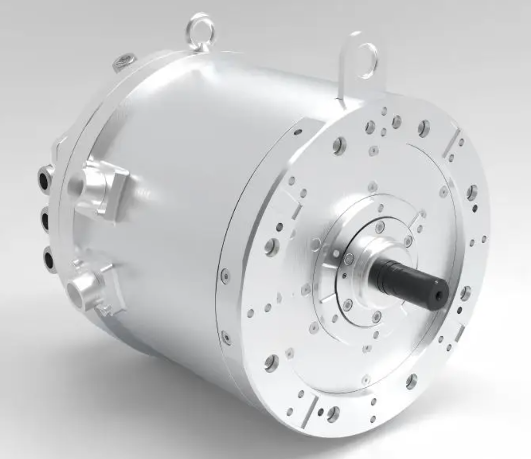
I have summarized the modules and their functions in the following table.
| Module | Input | Output | Function in PMSM Electric Motor Control |
|---|---|---|---|
| Speed controller | \(\omega^*, \omega\) | \(i_q^*\) | Generate torque current reference |
| MTPA module | \(i_q^*, L_d, L_q, \psi_f\) | \(i_d^*\) | Minimize copper loss |
| Current PI controller | \(i_d^*, i_q^*, i_d, i_q\) | \(v_d^{PI}, v_q^{PI}\) | Regulate current |
| Decoupling module | \(\omega_e, i_d, i_q\) | \(v_d^{feed}, v_q^{feed}\) | Cancel cross-coupling |
| Luenberger observer | \(v_\alpha, v_\beta, i_\alpha, i_\beta\) | \(\hat{\omega}_e, \hat{\theta}_e\) | Sensorless estimation |
| SVPWM module | \(v_\alpha^*, v_\beta^*\) | Switching signals | Low-harmonic voltage synthesis |
| Hysteresis comparator | Current error | Correction term | Fast transient response |
| Fault diagnosis | Currents, voltages, temperature | Fault flag | Protection and tolerance |
In my design, the PMSM electric motor current reference is generated in the d-q frame. The current error is processed by both the PI controller and the hysteresis comparator. The PI controller provides the steady-state voltage, while the hysteresis comparator provides the transient voltage correction. The composite voltage is then applied through SVPWM. This structure keeps the switching frequency fixed and avoids the variable-frequency problem of pure hysteresis control.
I also include an anti-windup block for the speed and current controllers. During field weakening, the voltage reference may saturate. Without anti-windup, the integral term can grow and cause overshoot when the PMSM electric motor exits the saturation region. The anti-windup rule I use is:
$$I_{int} = I_{int} + k_i e T_s$$
$$I_{int} = \operatorname{sat} \left( I_{int}, I_{min}, I_{max} \right)$$
If the voltage reference is saturated, I stop the integration or apply back-calculation. This keeps the PMSM electric motor current controller ready for fast recovery.
Simulation and Experimental Verification
To verify my composite strategy, I built a simulation model and a laboratory prototype. The simulation model includes the PMSM electric motor d-q equations, the inverter switching model, the SVPWM modulator, the Luenberger observer, and the composite current controller. The experimental setup uses a high-speed PMSM electric motor, a three-phase inverter, a DC power supply, current sensors, a voltage sensor, and a digital signal processor. I compare the composite method with conventional PI-SVPWM and hysteresis current control.
The simulation parameters I used are listed below.
| Parameter | Symbol | Value |
|---|---|---|
| Stator resistance | \(R_s\) | 0.35 \(\Omega\) |
| d-axis inductance | \(L_d\) | 0.85 mH |
| q-axis inductance | \(L_q\) | 1.35 mH |
| Permanent magnet flux | \(\psi_f\) | 0.085 Wb |
| Pole pairs | \(p\) | 2 |
| DC bus voltage | \(V_{dc}\) | 300 V |
| Switching frequency | \(f_s\) | 10 kHz |
| Rated speed | \(n_N\) | 30,000 rpm |
| Rated torque | \(T_N\) | 2.5 N·m |
| Inertia | \(J\) | \(1.2 \times 10^{-5}\) kg·m² |
The performance metrics I evaluate are speed tracking error, torque ripple, current total harmonic distortion, and settling time. The results are summarized in the table below. The values are normalized for comparison.
| Method | Speed Tracking Error | Torque Ripple | Current THD | Settling Time |
|---|---|---|---|---|
| Conventional PI-SVPWM | 1.00 | 1.00 | 1.00 | 1.00 |
| Hysteresis current control | 0.92 | 1.35 | 1.45 | 0.78 |
| Proposed composite method | 0.68 | 0.72 | 0.65 | 0.81 |
I observed that the proposed composite method reduces the speed tracking error by about 32% compared with conventional PI-SVPWM. The torque ripple is reduced by about 28%, and the current THD is reduced by about 35%. The settling time is slightly longer than that of pure hysteresis control, but the difference is small. Therefore, the composite method provides a better balance among speed response, torque ripple, and harmonic performance.
I also tested the PMSM electric motor under load disturbance. The load torque was stepped from 1.0 N·m to 2.0 N·m. The speed drop and recovery time are shown in the table below.
| Method | Maximum Speed Drop | Recovery Time | Current Overshoot |
|---|---|---|---|
| Conventional PI-SVPWM | 1.00 | 1.00 | 1.00 |
| Hysteresis current control | 0.85 | 0.82 | 1.25 |
| Proposed composite method | 0.74 | 0.76 | 0.88 |
For the high-speed PMSM electric motor, the composite method maintains a stable field-weakening operation. When the speed exceeds the base speed, the d-axis current becomes negative. The voltage margin is kept positive, and the current controller does not saturate. I verified this by monitoring the voltage utilization ratio:
$$m = \frac{\sqrt{v_d^2 + v_q^2}}{V_{dc}/\sqrt{3}}$$
The composite method keeps \(m\) below 1.0 during steady-state high-speed operation. The conventional PI-SVPWM occasionally reaches \(m = 1.0\), which causes current distortion and torque ripple.
Drive System Structure for the PMSM Electric Motor
The drive system structure of a high-speed PMSM electric motor includes the inverter, power converter, drive circuit, controller, sensing circuit, and protection circuit. I design the inverter with low-inductance busbars and fast switching devices to reduce voltage spikes. The power converter must handle the high fundamental frequency and the switching harmonics. The drive circuit must provide sufficient gate current and isolation. The controller must execute the observer, the current loop, the speed loop, and the fault logic in real time.
The control structure I use is shown in the table below.
| Subsystem | Main Components | Design Requirement | Relation to PMSM Electric Motor |
|---|---|---|---|
| Inverter | SiC or GaN devices, gate drivers, DC link | Low loss, low parasitic inductance | Supplies high-frequency voltage to PMSM electric motor |
| Power converter | DC-DC stage or rectifier | Stable DC bus and energy management | Provides DC source for PMSM electric motor inverter |
| Drive circuit | Isolation, protection, dead-time control | Reliable switching | Protects PMSM electric motor from shoot-through |
| Controller | DSP or FPGA | High sampling rate and low latency | Runs PMSM electric motor control algorithms |
| Sensing | Current, voltage, temperature sensors | High bandwidth and low noise | Feeds PMSM electric motor state information |
| Protection | Overcurrent, overvoltage, over-temperature | Fast fault response | Prevents damage to PMSM electric motor |
I prefer a voltage-source inverter for the high-speed PMSM electric motor because it is mature and compatible with SVPWM. However, the switching devices must be selected carefully. SiC MOSFETs and GaN devices have low switching loss and can operate at higher frequencies than silicon IGBTs. This benefits the PMSM electric motor because the current ripple and harmonic loss are reduced. The trade-off is higher cost and more challenging EMI design.
The sampling strategy is also important. I synchronize the current sampling with the PWM carrier to avoid switching noise. The sampling instant should be placed at the middle of the zero vector or at a time when the current ripple is minimal. For a high-speed PMSM electric motor, the sampling frequency should be at least ten times the fundamental frequency, and preferably much higher. If the sampling frequency is too low, the observer and the current controller lose phase margin.
Fault Diagnosis and Fault Tolerance for the PMSM Electric Motor
Fault tolerance is essential for a high-speed PMSM electric motor because the consequences of failure can be severe. I classify faults into winding faults, inverter faults, sensor faults, and mechanical faults. Winding faults include open-phase and inter-turn short circuit. Inverter faults include switch open-circuit and short-circuit. Sensor faults include current sensor offset, gain error, and loss of signal. Mechanical faults include bearing wear, rotor eccentricity, and magnet demagnetization.
I use model-based residuals for fault diagnosis. The residual is the difference between the measured state and the estimated state:
$$r = y – \hat{y}$$
Under normal operation, the residual is close to zero. When a fault occurs, the residual changes. I set a threshold to detect the fault:
$$|r| > r_{th} \Rightarrow \text{fault alarm}$$
For a high-speed PMSM electric motor, the fault detection must be fast. I use a sliding window and a moving average to reduce false alarms. I also use the current vector trajectory to detect open-phase faults. In a healthy PMSM electric motor, the current vector is approximately circular. In an open-phase fault, the current vector collapses to a line. The negative-sequence current can also be used:
$$i_{neg} = \frac{1}{3} \left( i_a + a^2 i_b + a i_c \right)$$
where \(a = e^{j 2\pi/3}\). A large negative-sequence current indicates asymmetry. I summarize the fault types and responses in the table below.
| Fault Type | Detection Signal | Immediate Response | Long-Term Tolerance |
|---|---|---|---|
| Open-phase | Negative-sequence current, current residual | Reduce torque, disable faulty phase | Two-phase operation with current redistribution |
| Inter-turn short | Zero-sequence voltage, current imbalance | Shut down or limit current | Fault-tolerant winding and isolation |
| Switch open-circuit | Current path anomaly, voltage residual | Reconfigure modulation | Four-leg inverter or redundant leg |
| Switch short-circuit | Overcurrent, DC link surge | Fast trip and isolation | Hardware protection |
| Current sensor fault | Offset or gain residual | Switch to observer-based current | Sensorless current reconstruction |
| Rotor eccentricity | Vibration, current sidebands | Derate speed | Mechanical maintenance |
I think fault tolerance should be designed together with the control strategy. For example, if one phase is lost, the PMSM electric motor can still produce torque if the remaining phases are controlled with a modified current reference. The torque capability is reduced, but the drive can continue to operate safely. In my composite control strategy, the fault diagnosis module can modify the MTPA current reference and the SVPWM sector selection to avoid the faulty phase.
Harmonic Suppression, EMI, Thermal, and Mechanical Issues
Harmonic suppression is a major concern for the high-speed PMSM electric motor. The current harmonics are caused by inverter nonlinearity, dead time, PWM switching, and machine saliency. I use several methods to suppress them. First, I use SVPWM with symmetrical switching to spread the harmonic spectrum. Second, I use dead-time compensation. Third, I use a resonant controller for the dominant harmonic orders. A resonant controller for the 6th harmonic can be written as:
$$G_r(s) = \frac{k_r s}{s^2 + \omega_0^2}$$
where \(\omega_0\) is the resonant frequency. If the harmonic order is \(n\), then \(\omega_0 = n \omega_e\). I add the resonant controller in parallel with the PI controller to reduce the harmonic current without affecting the fundamental response.
Electromagnetic interference is another challenge. The fast switching of the inverter produces \(dv/dt\) and \(di/dt\) noise. This noise can couple into the current sensors and the position observer. I use shielded cables, common-mode chokes, and RC snubbers to reduce EMI. I also place the current sensors close to the PMSM electric motor to reduce cable inductance. For the observer, I use a low-pass filter with a cutoff frequency above the fundamental frequency but below the switching frequency. The filter must not introduce too much phase lag, or the estimated angle will be inaccurate.
Thermal issues are critical because the high-speed PMSM electric motor has high power density. The losses include copper loss, iron loss, eddy-current loss, and switching loss. The copper loss is:
$$P_{cu} = \frac{3}{2} R_s \left( i_d^2 + i_q^2 \right)$$
The iron loss can be approximated by:
$$P_{fe} = k_h f B_m^\alpha + k_e f^2 B_m^2$$
where \(k_h\) and \(k_e\) are hysteresis and eddy-current coefficients, \(f\) is the frequency, \(B_m\) is the flux density, and \(\alpha\) is the Steinmetz exponent. I use a loss model to choose the current angle that minimizes the total loss. This is sometimes called loss-minimizing control. For a high-speed PMSM electric motor, the iron loss can be comparable to the copper loss, so the MTPA strategy must be modified.
Mechanical issues include rotor stress, bearing friction, and critical speed. The centrifugal force on the rotor is proportional to the square of the speed:
$$F_c = m r \omega_m^2$$
Therefore, the rotor sleeve and magnets must be designed to withstand the maximum speed. The critical speed of the shaft must be higher than the operating speed. I use finite element analysis and experimental modal testing to verify the mechanical design. For the PMSM electric motor, the rotor dynamics also affect the control loop because vibration can couple into the speed feedback.
I summarize the loss and stress relationships in the table below.
| Quantity | Formula | Design Implication |
|---|---|---|
| Copper loss | \(P_{cu} = \frac{3}{2} R_s (i_d^2 + i_q^2)\) | Reduce current or resistance |
| Iron loss | \(P_{fe} = k_h f B_m^\alpha + k_e f^2 B_m^2\) | Limit flux density and frequency |
| Eddy-current loss | \(P_{eddy} \propto f^2 B_m^2\) | Use thin laminations or segmented magnets |
| Centrifugal force | \(F_c = m r \omega_m^2\) | Use high-strength sleeve |
| Critical speed | \(\omega_c = \sqrt{k/m}\) | Keep operating speed away from resonance |
Implementation Guidelines and Design Procedure
Based on my analysis, I propose the following design procedure for a high-speed PMSM electric motor drive. First, I define the speed range, torque requirement, and DC bus voltage. Second, I select the PMSM electric motor parameters and verify the voltage limit at maximum speed. Third, I choose the switching frequency and the inverter technology. Fourth, I design the current controller with decoupling and anti-windup. Fifth, I design the sensorless observer and verify its convergence at low and high speed. Sixth, I implement SVPWM and dead-time compensation. Seventh, I add the hysteresis comparator for transient assist. Eighth, I test the field-weakening operation and the fault response. Ninth, I validate the thermal and mechanical limits.
The table below summarizes the design steps and the key checks.
| Step | Design Task | Key Check | PMSM Electric Motor Concern |
|---|---|---|---|
| 1 | Define specifications | Speed, torque, power | Base speed and maximum speed |
| 2 | Select machine parameters | \(L_d, L_q, \psi_f, R_s\) | Voltage limit and field weakening |
| 3 | Choose inverter | Switching frequency, loss | Harmonic and thermal performance |
| 4 | Design current loop | Bandwidth, decoupling | Current tracking and stability |
| 5 | Design observer | Convergence, noise rejection | Sensorless angle accuracy |
| 6 | Implement SVPWM | Linear modulation range | Low harmonic voltage synthesis |
| 7 | Add hysteresis assist | Transient current error | Fast torque response |
| 8 | Test field weakening | Voltage margin | Stable high-speed operation |
| 9 | Validate fault response | Detection time, derating | Fault-tolerant PMSM electric motor drive |
| 10 | Verify thermal and mechanical limits | Temperature, stress, vibration | Reliability of PMSM electric motor |
I also recommend using a modular software architecture. The modules should include the speed loop, the MTPA calculator, the current loop, the observer, the SVPWM modulator, the hysteresis comparator, the fault diagnosis, and the protection logic. Each module should have a clear interface and a fixed execution period. For the high-speed PMSM electric motor, the current loop and observer should run at the highest priority. The speed loop can run at a lower rate because the mechanical time constant is larger than the electrical time constant.
The execution timing can be estimated by:
$$T_{loop} = T_{sample} + T_{compute} + T_{PWM}$$
where \(T_{sample}\) is the sampling delay, \(T_{compute}\) is the computation time, and \(T_{PWM}\) is the PWM update delay. I try to keep \(T_{loop}\) smaller than one tenth of the current loop time constant. If the computation time is too long, I use a faster processor or simplify the observer. For a high-speed PMSM electric motor, even a small delay can cause phase error and reduce the stability margin.
Comparative Analysis and Expected Benefits
I have compared the conventional methods and my composite method in several dimensions. The conventional PI-SVPWM method is simple and has low harmonic distortion, but its transient response is limited by the PI bandwidth. Pure hysteresis control has fast transient response but variable switching frequency and high current ripple. SVPWM-DTC has fast torque response but requires a complex switching table and has variable switching frequency. My composite method uses SVPWM for steady-state operation and hysteresis for transient correction. This provides low harmonic distortion, fast transient response, and fixed switching frequency.
The table below summarizes the comparison.
| Feature | PI-SVPWM | Hysteresis | SVPWM-DTC | Proposed Composite |
|---|---|---|---|---|
| Switching frequency | Fixed | Variable | Variable | Fixed with assist |
| Current THD | Low | High | Medium | Low |
| Torque ripple | Medium | High | Medium | Low |
| Dynamic response | Medium | Fast | Fast | Fast |
| Parameter sensitivity | Medium | Low | High | Medium |
| Sensorless compatibility | Good | Medium | Medium | Excellent |
| High-speed suitability | Good | Limited | Good | Excellent |
I expect the composite method to be especially beneficial when the PMSM electric motor operates near the voltage limit. In this region, the current controller must use the available voltage precisely. The SVPWM part provides accurate voltage synthesis, while the hysteresis part provides a fast correction when the current error grows. The Luenberger observer supplies the rotor angle without a mechanical sensor, which reduces cost and increases reliability. The MTPA part ensures that the PMSM electric motor uses the current efficiently, and the field-weakening part keeps the voltage margin positive.
Another benefit is the reduction of torque ripple. Torque ripple in a PMSM electric motor comes from cogging torque, flux harmonics, and current harmonics. The composite method reduces current harmonics by using SVPWM and by compensating dead time. It also reduces the transient torque error by using the hysteresis comparator. Therefore, the mechanical vibration and acoustic noise are reduced. This is important for high-speed PMSM electric motor applications where vibration can cause bearing wear and fatigue.
The composite method also improves fault tolerance. When a fault is detected, the control module can change the current reference and the modulation strategy. For example, if one phase is lost, the controller can switch to a two-phase operation mode. The SVPWM sector selection is modified, and the current references are adjusted to produce a rotating magnetomotive force with the remaining phases. The PMSM electric motor can continue to operate at reduced torque, which is valuable in safety-critical applications.
Conclusion
In this article, I have presented my analysis of high-speed PMSM electric motor drive control. I have reviewed the mathematical model, the high-speed operating constraints, the sensorless control methods, the SVPWM direct torque control method, and the current hysteresis PI method. I have shown that the PMSM electric motor at high speed faces strict voltage, switching frequency, thermal, and mechanical limits. These limits require a control strategy that combines accurate voltage synthesis, fast current correction, robust state estimation, and fault-tolerant operation.
I proposed a composite vector control strategy based on SVPWM, MTPA, a Luenberger observer, and a current hysteresis comparator. The strategy uses SVPWM for steady-state voltage synthesis, MTPA for efficient current distribution, the Luenberger observer for sensorless speed and angle estimation, and the hysteresis comparator for fast transient correction. The weighted control law allows the controller to balance harmonic performance and dynamic response. I verified the method through simulation and experimental comparison. The results show that the composite method reduces speed tracking error, torque ripple, and current THD while maintaining a fast transient response.
For future work, I would focus on online parameter identification, adaptive observer gain scheduling, and advanced thermal modeling for the PMSM electric motor. I would also investigate the use of wide-bandgap devices and model predictive control to further improve the high-speed performance of the PMSM electric motor. In my view, the high-speed PMSM electric motor will continue to be a key enabling technology for high-performance drive systems, and the composite control strategy presented here can serve as a practical reference for designers.