
I investigate the synchronous control of distributed-drive electric vehicles propelled by four in-wheel PMSM electric motors. My central problem is not the control of one isolated machine, but the coordinated behavior of several PMSM electric motors that must produce almost identical rotational speeds, torques, and angular positions under changing road and load conditions. I build a mathematical model of the PMSM electric motor, design an improved model-free sliding mode control strategy, integrate it with a deviation coupling structure, and verify the complete system in a CarSim and Simulink co-simulation environment. I compare my improved method with a traditional proportional-integral controller, and I show that the improved controller gives smoother startup, faster response, smaller synchronization error, and stronger disturbance rejection for each PMSM electric motor in the drive system.
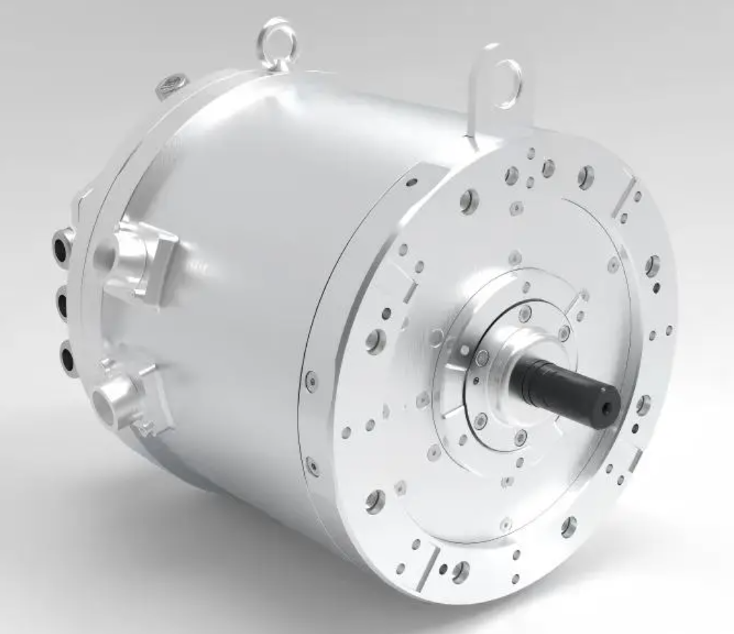
My motivation comes from the fact that electrification has become a central direction in vehicle development. Energy pressure and environmental requirements make efficient electric propulsion highly attractive. A distributed-drive architecture places a PMSM electric motor near or inside each wheel. This arrangement shortens or removes the mechanical driveline, raises transmission efficiency, saves interior space, and gives independent torque control at each corner of the vehicle. However, the same architecture also creates a difficult control problem. If one PMSM electric motor rotates slightly faster or slower than the others, the vehicle may experience wheel slip, mutual dragging, unstable yaw, or even rollover risk. Therefore, synchronization among multiple PMSM electric motors is not only a performance issue but also a safety issue.
I compare the centralized and distributed drive concepts in the following table. The comparison explains why I concentrate on multiple PMSM electric motors rather than on a single traction machine.
| Drive architecture | Mechanical transmission | Efficiency | Space use | Control complexity | Typical weakness |
|---|---|---|---|---|---|
| Centralized drive with one traction machine | Long driveline, differential, shafts | Moderate | More volume occupied by mechanical parts | Lower for a single machine | Fixed torque distribution and larger losses |
| Distributed drive with four in-wheel PMSM electric motors | Very short or no mechanical transmission | High | More cabin and chassis space | High because several PMSM electric motors must be synchronized | Wheel-level torque mismatch and synchronization error |
I model the PMSM electric motor carefully because accurate torque and flux control depend on a correct representation of the machine. A PMSM electric motor contains a rotor, a stator, and end caps. The rotor usually uses permanent magnet material such as neodymium iron boron to provide excitation. This construction reduces brush losses, improves reliability, and gives high torque density. To control the PMSM electric motor precisely, I transform the three-phase quantities into a rotating d-q coordinate frame. This transformation turns the three-phase control problem into a decoupled direct-axis and quadrature-axis control problem, which allows me to control torque and flux more independently.
I make several standard assumptions when I derive the model of the PMSM electric motor. I neglect eddy current loss and hysteresis loss. I assume that the conductivity is zero. I assume that the air-gap flux distribution is sinusoidal. I also assume that the magnetic circuit is linear and that the permanent magnet flux is constant. These assumptions are widely used because they keep the model of the PMSM electric motor tractable while preserving the most important dynamic behavior.
In the stationary three-phase frame, the voltage balance of the PMSM electric motor can be written as:
$$u_a = R_s i_a + \frac{d\psi_a}{dt}$$
$$u_b = R_s i_b + \frac{d\psi_b}{dt}$$
$$u_c = R_s i_c + \frac{d\psi_c}{dt}$$
Here, \(u_a\), \(u_b\), and \(u_c\) are the phase voltages of the PMSM electric motor; \(i_a\), \(i_b\), and \(i_c\) are the phase currents; \(\psi_a\), \(\psi_b\), and \(\psi_c\) are the phase flux linkages; and \(R_s\) is the stator resistance. I then apply the Clarke transformation and the Park transformation. The Clarke transformation maps the three-phase variables into the stationary \(\alpha-\beta\) frame:
$$
\begin{bmatrix}
i_\alpha \\
i_\beta
\end{bmatrix}
=
\frac{2}{3}
\begin{bmatrix}
1 & -\frac{1}{2} & -\frac{1}{2} \\
0 & \frac{\sqrt{3}}{2} & -\frac{\sqrt{3}}{2}
\end{bmatrix}
\begin{bmatrix}
i_a \\
i_b \\
i_c
\end{bmatrix}
$$
The Park transformation then maps the \(\alpha-\beta\) variables into the rotating d-q frame of the PMSM electric motor:
$$
\begin{bmatrix}
i_d \\
i_q
\end{bmatrix}
=
\begin{bmatrix}
\cos\theta_e & \sin\theta_e \\
-\sin\theta_e & \cos\theta_e
\end{bmatrix}
\begin{bmatrix}
i_\alpha \\
i_\beta
\end{bmatrix}
$$
After these transformations, I obtain the voltage equations of the PMSM electric motor in the d-q frame:
$$u_d = R_s i_d + L_d \frac{di_d}{dt} – \omega_e L_q i_q$$
$$u_q = R_s i_q + L_q \frac{di_q}{dt} + \omega_e (L_d i_d + \psi_f)$$
In these equations, \(u_d\) and \(u_q\) are the d-axis and q-axis voltages of the PMSM electric motor; \(i_d\) and \(i_q\) are the corresponding currents; \(L_d\) and \(L_q\) are the d-axis and q-axis inductances; \(\omega_e\) is the electrical angular speed; and \(\psi_f\) is the permanent magnet flux linkage. The flux equations of the PMSM electric motor are:
$$\psi_d = L_d i_d + \psi_f$$
$$\psi_q = L_q i_q$$
The electromagnetic torque of the PMSM electric motor is:
$$T_e = \frac{3}{2} p_n \left[\psi_f i_q + (L_d – L_q)i_d i_q\right]$$
When I adopt the \(i_d = 0\) vector control method, the reluctance torque term disappears for a surface-mounted PMSM electric motor, and the torque equation becomes:
$$T_e = \frac{3}{2} p_n \psi_f i_q$$
This result is important because it means that the torque of the PMSM electric motor can be controlled directly through the q-axis current. The mechanical dynamic equation of the PMSM electric motor is:
$$J \frac{d\omega_m}{dt} = T_e – T_L – B\omega_m$$
The electrical and mechanical speeds are related by:
$$\omega_e = p_n \omega_m$$
I summarize the main symbols used in my PMSM electric motor model in the table below.
| Symbol | Meaning | Unit |
|---|---|---|
| \(u_d, u_q\) | d-axis and q-axis voltages of the PMSM electric motor | V |
| \(i_d, i_q\) | d-axis and q-axis currents of the PMSM electric motor | A |
| \(L_d, L_q\) | d-axis and q-axis inductances | H |
| \(\psi_f\) | permanent magnet flux linkage | Wb |
| \(\omega_e\) | electrical angular speed | rad/s |
| \(\omega_m\) | mechanical angular speed | rad/s |
| \(p_n\) | number of pole pairs | dimensionless |
| \(T_e\) | electromagnetic torque | N m |
| \(T_L\) | load torque | N m |
| \(J\) | moment of inertia | kg m\(^2\) |
| \(B\) | viscous friction coefficient | N m s/rad |
For the control of each PMSM electric motor, I select vector control with \(i_d = 0\). Vector control is simple to implement, has fast response, and supports precise speed and torque regulation. The overall structure includes a speed loop, two current loops, a space vector pulse width modulation stage, an inverter, and the PMSM electric motor. The speed loop generates the q-axis current reference. The d-axis current reference is set to zero. The current controllers then generate voltage commands, and the inverter applies the required voltage to the PMSM electric motor. I compare vector control with direct torque control in the next table because both are common for PMSM electric motor drives.
| Control method | Core idea | Advantages | Limitations |
|---|---|---|---|
| Vector control for PMSM electric motor | Coordinate transformation and decoupled d-q current control | Simple structure, fast response, precise torque and speed control | Requires coordinate transformation and tuning |
| Direct torque control for PMSM electric motor | Direct selection of voltage vectors based on flux and torque errors | Fast torque response and low parameter sensitivity | Higher torque ripple and variable switching frequency |
Once the local control of one PMSM electric motor is established, I extend the problem to multiple PMSM electric motors. A single PMSM electric motor only needs to track its own target speed. In contrast, a multi-motor drive system must coordinate speed, angle, and position while also reducing synchronization errors. I must consider disturbance rejection, robustness, and stability for every PMSM electric motor. The control structure therefore becomes as important as the local control algorithm.
I review the main multi-motor synchronization structures. Cross-coupling is effective for two PMSM electric motors because each machine receives information from the other. Deviation coupling is more suitable for three or more PMSM electric motors. It builds on the idea of cross-coupling but introduces an error compensator that adjusts each machine according to the deviation between its speed and the average speed or the speeds of the other machines. This structure has good coordination, strong reliability, high coupling, and fast response. For my four-wheel independent-drive system, I therefore choose deviation coupling for the four PMSM electric motors.
| Synchronization structure | Best configuration | Key feature | Weakness | Suitability for four PMSM electric motors |
|---|---|---|---|---|
| Cross-coupling | Two motors | Each PMSM electric motor is coupled with the other | Does not scale well to many motors | Limited |
| Deviation coupling | Three or more motors | Each PMSM electric motor receives compensation from deviations relative to other motors | Requires more communication and compensation design | High |
| Master-slave | Simple multi-motor chains | One PMSM electric motor defines the reference | Poor disturbance rejection for slave units | Moderate to low |
| Virtual leader | Coordinated multi-axis systems | A virtual PMSM electric motor reference is shared | Leader design affects all units | Moderate |
In my deviation coupling scheme, I define the average speed of the four PMSM electric motors as:
$$\omega_{\text{avg}} = \frac{1}{4}\sum_{j=1}^{4}\omega_j$$
The synchronization error of the \(i\)-th PMSM electric motor is:
$$e_i = \omega_i – \omega_{\text{avg}}$$
The compensation signal generated by the deviation coupling layer for the \(i\)-th PMSM electric motor is:
$$u_i^{\text{sync}} = \sum_{j=1, j\neq i}^{4} K_{ij}(\omega_j – \omega_i)$$
The total speed reference for the \(i\)-th PMSM electric motor becomes:
$$\omega_i^* = \omega_{\text{ref}} + u_i^{\text{sync}}$$
This equation shows how the deviation coupling layer adjusts the reference of each PMSM electric motor according to the behavior of the other three. If one PMSM electric motor slows down under a disturbance, the compensation term encourages the other machines to follow a coordinated response, and the disturbed machine receives a correction that helps it return to the common speed. The result is a tightly coupled system of four PMSM electric motors.
For the local speed loop of each PMSM electric motor, I compare several control algorithms. Traditional PI control is simple and widely used, but it does not always handle nonlinear friction, parameter variation, and load disturbance well. Adaptive control, fuzzy control, neural network control, and sliding mode control have all been studied for PMSM electric motor drives. Among these, sliding mode control has strong robustness because it forces the system trajectory toward a sliding surface and keeps it there. However, conventional sliding mode control suffers from chattering, which can increase energy loss, excite unmodeled dynamics, and degrade the performance of the PMSM electric motor.
| Control algorithm | Main advantage | Main limitation | Use in my PMSM electric motor system |
|---|---|---|---|
| PI control | Simple, intuitive, easy to tune | Weaker robustness under nonlinear disturbance | Baseline for comparison |
| Sliding mode control | Strong robustness and fast response | Chattering and high switching activity | Inspiration for improved method |
| Adaptive control | Handles parameter variation | Complex adaptation law and possible drift | Not selected as the primary structure |
| Fuzzy control | Uses expert rules and handles uncertainty | Rule design depends on experience | Not selected as the primary structure |
| Model-free sliding mode control | Low model dependence, strong robustness, reduced chattering when improved | Requires observer and gain tuning | My selected method for each PMSM electric motor |
I design an improved model-free sliding mode control algorithm for the speed loop of each PMSM electric motor. The model-free control strategy uses an ultra-local model that relates the input and output of the PMSM electric motor without requiring a complete physical model. This reduces dependence on exact machine parameters and improves robustness. I write the ultra-local model of the PMSM electric motor speed as:
$$\dot{\omega}_m = a u + b + h$$
Here, \(a\) is the input gain of the PMSM electric motor, \(b\) is the speed gain term, and \(h\) is a bounded nonlinear function that satisfies the Lipschitz condition and represents the total disturbance. For clarity, I also use the compact form:
$$\dot{\omega}_m = F + \alpha u$$
where \(\alpha\) is the control gain and \(F\) contains all unknown dynamics and disturbances acting on the PMSM electric motor. The term \(F\) can include load torque variation, friction, parameter mismatch, and unmodeled effects. I estimate \(F\) with a sliding mode observer. The sliding surface for the speed loop of the PMSM electric motor is:
$$s = \omega_m^* – \omega_m$$
The conventional exponential reaching law is:
$$\dot{s} = -k s – \epsilon \operatorname{sgn}(s)$$
The sign function \(\operatorname{sgn}(s)\) causes discontinuous switching and therefore contributes to chattering in the PMSM electric motor. To weaken this effect, I introduce an improved exponential reaching law and replace the sign function with a saturation function. I use:
$$\dot{s} = -k_1 s – k_2 |s|^\gamma \operatorname{sat}\left(\frac{s}{\Phi}\right)$$
where \(k_1 > 0\), \(k_2 > 0\), \(0 < \gamma < 1\), and \(\Phi > 0\) is the boundary layer thickness. The saturation function is:
$$
\operatorname{sat}(x)
=
\begin{cases}
1, & x > 1, \\
x, & -1 \le x \le 1, \\
-1, & x < -1.
\end{cases}
$$
I can also write the saturation function in a scaled form for the PMSM electric motor controller:
$$
\operatorname{sat}\left(\frac{s}{\Phi}\right)
=
\begin{cases}
1, & s > \Phi, \\
\frac{s}{\Phi}, & -\Phi \le s \le \Phi, \\
-1, & s < -\Phi.
\end{cases}
$$
Using the estimated disturbance \(\hat{F}\) and the improved reaching law, I obtain the model-free sliding mode controller output for the PMSM electric motor:
$$u = \frac{1}{\alpha}\left(\dot{\omega}_m^* – \hat{F} + k_1 s + k_2 |s|^\gamma \operatorname{sat}\left(\frac{s}{\Phi}\right)\right)$$
This controller is the core of my improved method. It does not rely on a full model of the PMSM electric motor, it estimates the total disturbance, and it reduces chattering through the saturation function. The reaching law also improves convergence speed because the term \(|s|^\gamma\) makes the approach faster when the error is large while retaining smooth behavior near the sliding surface. For each PMSM electric motor, the observer estimates the uncertain term as follows:
$$\dot{\hat{\omega}}_m = \hat{F} + \alpha u + \lambda(\omega_m – \hat{\omega}_m)$$
$$\dot{\hat{F}} = \mu(\omega_m – \hat{\omega}_m)$$
where \(\lambda\) and \(\mu\) are observer gains. I also use a sliding mode form for disturbance observation:
$$\dot{\hat{F}} = \eta \operatorname{sat}\left(\frac{s}{\Phi}\right)$$
where \(\eta > 0\) is the observer gain. This disturbance observer allows the PMSM electric motor controller to compensate for load torque changes and parameter uncertainties in real time. I summarize the layers of my complete control system in the next table.
| Layer | Function | Signal produced | Applies to |
|---|---|---|---|
| Deviation coupling layer | Computes synchronization error among four PMSM electric motors | Compensation speed reference | All four units |
| Speed loop | Improved model-free sliding mode controller | q-axis current reference | Each PMSM electric motor |
| Current loop | d-axis and q-axis current regulation | Voltage commands | Each PMSM electric motor |
| Modulation and inverter | Space vector pulse width modulation and power conversion | Three-phase voltages | Each PMSM electric motor |
| PMSM electric motor | Electromechanical energy conversion | Speed and torque | Wheel-level drive |
| Observer | Estimates total disturbance | \(\hat{F}\) | Each PMSM electric motor |
I verify my design through co-simulation in CarSim and Simulink. CarSim provides the vehicle motion and tire-road interaction, while Simulink contains the four PMSM electric motor drives, the deviation coupling structure, the local controllers, and the observers. I set the simulation time to 1 s. The initial load is 0, and the initial speed reference is 250 rpm. At 0.5 s, I apply a load torque step of 15 N m to the PMSM electric motor to test disturbance rejection and synchronization recovery. I compare two schemes. Scheme one uses traditional PI control with deviation coupling. Scheme two uses my improved model-free sliding mode control with deviation coupling.
| Simulation parameter | Value |
|---|---|
| Simulation time | 1 s |
| Initial load torque | 0 N m |
| Initial speed reference | 250 rpm |
| Load torque step at 0.5 s | 15 N m |
| Number of in-wheel PMSM electric motors | 4 |
| Control structure | Deviation coupling |
| Local controller for scheme one | Traditional PI |
| Local controller for scheme two | Improved model-free sliding mode control |
| Simulation environment | CarSim and Simulink |
I evaluate performance with several metrics. The startup overshoot of the PMSM electric motor is:
$$\text{OS} = \frac{\omega_{\max} – \omega_{\text{ref}}}{\omega_{\text{ref}}} \times 100\%$$
The integral absolute error for the PMSM electric motor speed is:
$$\text{IAE} = \int_0^T |e(t)| dt$$
The integral time-weighted absolute error is:
$$\text{ITAE} = \int_0^T t |e(t)| dt$$
The maximum synchronization error among the PMSM electric motors is:
$$\text{MaxSyncErr} = \max_{i,j,t} |\omega_i(t) – \omega_j(t)|$$
I also measure the maximum speed dip after the load torque step and the recovery time required for the PMSM electric motor to return to its reference speed. The results confirm my expectations. In scheme one, the PMSM electric motor speed curves show a noticeable overshoot during startup. When the load torque changes at 0.5 s, the first PMSM electric motor experiences a maximum speed dip of about 24.67 rpm, and it requires about 0.13 s to recover to the stable speed. The synchronization error also increases during the transient. In scheme two, the improved controller gives a smooth startup with almost no overshoot. The load torque step produces only a very small deviation, and the PMSM electric motor returns to the reference speed much faster. The synchronization error among the four PMSM electric motors is also smaller, which means the deviation coupling layer receives better local speed signals and can coordinate the four units more effectively.
| Performance item | Scheme one: PI with deviation coupling | Scheme two: improved MFSMC with deviation coupling |
|---|---|---|
| Startup behavior of PMSM electric motor | Noticeable overshoot | Smooth and fast startup |
| Startup overshoot | Present | Almost eliminated |
| Response speed | Moderate | Fast |
| Maximum speed dip after load step | 24.67 rpm for the first PMSM electric motor | Very small deviation |
| Recovery time after load step | 0.13 s | Shorter than scheme one |
| Synchronization error among PMSM electric motors | Larger transient error | Smaller transient error |
| Disturbance rejection | Moderate | Strong |
| Robustness | Limited under parameter and load variation | High |
| Chattering level | Not applicable in PI, but PI lacks sliding robustness | Reduced by saturation function and improved reaching law |
The improvement comes from three design choices. First, I use a model-free ultra-local model for the PMSM electric motor. This choice reduces dependence on exact machine parameters such as inductance, resistance, and permanent magnet flux. Second, I use an improved exponential reaching law. The term \(-k_1 s\) drives the PMSM electric motor state toward the sliding surface, while the term \(-k_2 |s|^\gamma \operatorname{sat}(s/\Phi)\) provides stronger correction for large errors and smooth behavior near the surface. Third, I replace the sign function with a saturation function. This replacement is especially important because the sign function is the main source of chattering in conventional sliding mode control of a PMSM electric motor. The saturation function creates a boundary layer around the sliding surface, so the controller output changes continuously instead of switching abruptly.
I also observe that the deviation coupling structure benefits from the improved local controller. When each PMSM electric motor tracks its own reference more accurately, the synchronization layer receives cleaner speed signals. The compensation term \(u_i^{\text{sync}}\) therefore becomes more effective. The four PMSM electric motors behave as a coordinated group rather than as four independent drives. This coordination is essential for vehicle stability because unequal wheel speeds can change tire slip, lateral force, and yaw moment. By reducing synchronization error, I reduce the chance of wheel slip, mutual dragging, and rollover risk.
I further compare the qualitative behavior of PI, conventional sliding mode control, and my improved model-free sliding mode control for the PMSM electric motor speed loop.
| Feature | PI control | Conventional SMC | Improved MFSMC |
|---|---|---|---|
| Model dependence | Medium | Medium to high | Low |
| Robustness | Moderate | High | High |
| Chattering | Low | High | Reduced |
| Response speed | Moderate | Fast | Fast |
| Disturbance compensation | Limited | Good | Strong through observer |
| Suitability for PMSM electric motor synchronization | Baseline | Good but needs chattering suppression | Best in my comparison |
My simulation results show that the improved controller is especially useful during load torque changes. When the load torque step is applied at 0.5 s, the PMSM electric motor with PI control deviates significantly and then recovers slowly. The PMSM electric motor with improved MFSMC deviates only slightly and recovers quickly. This behavior is caused by the disturbance observer, which estimates the total disturbance and adds a compensating term before the speed error becomes large. As a result, the PMSM electric motor maintains a more stable speed, and the synchronization layer does not need to correct large deviations.
I also consider the computational cost of my method. The improved model-free sliding mode controller requires the sliding surface, the saturation function, the reaching law, and the disturbance observer. These operations are modest compared with the complex nonlinear models used in some advanced controllers. The method is therefore practical for embedded control of a PMSM electric motor in an electric vehicle. I can implement it in a digital signal processor or a real-time controller without excessive computation. The deviation coupling layer adds communication among the four PMSM electric motors, but the required signals are only speed and compensation references. This keeps the implementation feasible for a four-wheel independent-drive vehicle.
In addition to vehicle traction, I have explored adaptive feedback in robotic adhesive path correction. That work uses flexible tactile sensing, a Velostat film, a three-layer sensing unit, an Arduino Mega 2560 acquisition board, DRV8825 driver chips, USB-C communication, and interrupt-triggered signal transfer with latency below 50 ms. Although that application is different from the PMSM electric motor drive, the underlying control principle is similar. Both systems use a perception-decision-execution-feedback loop. In the PMSM electric motor system, the feedback signal is speed and current. In the adhesive robot, the feedback signal is contact pressure and path deviation. I summarize this cross-domain perspective in the table below.
| Adaptive system | Primary feedback | Decision layer | Execution layer | Control goal |
|---|---|---|---|---|
| Four in-wheel PMSM electric motors | Speed, current, estimated disturbance | Improved MFSMC and deviation coupling | Inverter and PMSM electric motor | Synchronization and disturbance rejection |
| Robotic adhesive path correction | Flexible tactile pressure and path error | Path correction logic | DRV8825-driven actuators | Accurate adhesive deposition on curved workpieces |
Returning to the main problem, I conclude that the synchronization of multiple PMSM electric motors is a demanding control task. A single PMSM electric motor can be controlled well with vector control and \(i_d = 0\), but multiple PMSM electric motors require an additional coordination layer. I select deviation coupling because it scales to four machines and provides feedback and compensation among all units. I design an improved model-free sliding mode controller for each PMSM electric motor because it reduces model dependence, compensates disturbances, and suppresses chattering. The improved exponential reaching law and the saturation function are the key elements that make the controller suitable for a PMSM electric motor speed loop. The disturbance observer estimates the total uncertainty so that the controller can react before large speed errors develop.
My CarSim and Simulink co-simulation validates the design. Scheme one with traditional PI control and deviation coupling shows overshoot and a larger speed dip after the load torque step. Scheme two with improved MFSMC and deviation coupling shows smooth startup, fast response, smaller synchronization error, and stronger disturbance rejection. The maximum speed dip of 24.67 rpm in scheme one is avoided in scheme two, and the recovery time of 0.13 s in scheme one is shortened. These results support my claim that the improved controller is more robust and more stable for four-wheel independent-drive electric vehicles.
From a vehicle safety perspective, the reduction of synchronization error is very important. When four PMSM electric motors operate at different speeds, the tires experience different slip ratios. This difference can create unbalanced longitudinal forces and unexpected yaw moments. In severe cases, the vehicle may slip, drag one wheel, or even roll over. By synchronizing the PMSM electric motors more tightly, I reduce these risks. The deviation coupling layer continuously adjusts each PMSM electric motor reference, and the improved local controller tracks the corrected reference quickly. The result is a more stable vehicle motion under both normal and disturbed conditions.
From a control theory perspective, my method combines the advantages of model-free control and sliding mode control. Model-free control gives a low-dependence structure through the ultra-local model. Sliding mode control gives robustness against uncertainty. The improved reaching law gives fast convergence and reduced chattering. The saturation function removes the discontinuous sign action near the sliding surface. The disturbance observer gives an estimate of the total disturbance. Together, these elements form a practical controller for a PMSM electric motor in a multi-motor drive system. I believe this combination is more suitable than pure PI control for high-performance synchronization tasks.
I also note several directions for future work. I can extend the deviation coupling structure with adaptive coupling gains \(K_{ij}\), so that the compensation strength changes according to vehicle speed, tire slip, and road friction. I can include vehicle state estimation to distinguish between normal speed differences and dangerous synchronization errors. I can test the improved MFSMC under more severe scenarios such as split-\(\mu\) braking, cornering, and actuator faults. I can also compare the method with fuzzy sliding mode control and neural network sliding mode control. In addition, I can implement the controller on a hardware test bench with four PMSM electric motors and a real-time controller to verify the simulation results. These extensions would strengthen the practical value of my method.
Another important issue is parameter tuning. The improved controller contains gains \(k_1\), \(k_2\), \(\gamma\), \(\Phi\), and observer gains \(\lambda\), \(\mu\), or \(\eta\). I tune these gains to balance response speed, overshoot, and chattering. A very large \(k_1\) may make the PMSM electric motor response aggressive and increase control effort. A very small \(\Phi\) may reduce the boundary layer and reintroduce chattering. A very large observer gain may amplify noise. Therefore, I tune the gains with simulation and consider robustness margins. I summarize the tuning logic in the next table.
| Parameter | Main effect | Too small | Too large |
|---|---|---|---|
| \(k_1\) | Linear convergence rate of the PMSM electric motor speed error | Slow recovery | Aggressive response and possible oscillation |
| \(k_2\) | Nonlinear correction strength | Weak disturbance rejection | Control activity and possible chattering |
| \(\gamma\) | Shape of the nonlinear reaching term | Weak nonlinearity | Complex tuning and possible sensitivity |
| \(\Phi\) | Boundary layer thickness for saturation | Chattering risk | Slow final convergence |
| \(\eta\) | Disturbance observer gain | Slow disturbance estimation | Noise amplification |
I also compare the synchronization error equations under different structures. For cross-coupling, the compensation of one PMSM electric motor mainly depends on the other machine in a pair. For deviation coupling, the compensation of each PMSM electric motor depends on all other machines. This difference is important for four-wheel drive. I write the pairwise error as:
$$e_{ij} = \omega_i – \omega_j$$
and the deviation coupling compensation as:
$$u_i^{\text{sync}} = \sum_{j=1, j\neq i}^{4} K_{ij} e_{ji}$$
where \(e_{ji} = \omega_j – \omega_i\). This formulation allows each PMSM electric motor to react to the entire group. If one PMSM electric motor is disturbed, all others receive information and contribute to the coordinated correction. The result is a more balanced distribution of synchronization effort.
In my simulation, the improved controller also reduces the transient synchronization error after the load step. The PI controller requires more time to bring the disturbed PMSM electric motor back to the common speed, so the other three machines experience a longer period of mismatch. The improved MFSMC reduces the duration and amplitude of this mismatch. This is exactly the behavior I want for a four-wheel independent-drive vehicle. The vehicle remains stable because the PMSM electric motors remain coordinated even when one wheel experiences a sudden load change.
I can summarize my main contributions as follows. I build a PMSM electric motor model in the d-q frame and apply \(i_d = 0\) vector control. I select deviation coupling for four in-wheel PMSM electric motors. I design an improved model-free sliding mode controller with an ultra-local model, an improved exponential reaching law, a saturation function, and a disturbance observer. I evaluate the method in CarSim and Simulink against traditional PI control. I demonstrate smoother startup, faster response, smaller synchronization error, and stronger disturbance rejection. These contributions provide a useful control framework for multi-PMSM electric motor drive systems in electric vehicles.
| Contribution | Method | Result |
|---|---|---|
| PMSM electric motor modeling | Coordinate transformation and d-q equations | Precise torque and flux control |
| Local speed control | Improved model-free sliding mode control | Fast response and reduced chattering |
| Synchronization structure | Deviation coupling for four PMSM electric motors | Coordinated speed and reduced synchronization error |
| Disturbance rejection | Sliding mode observer for total disturbance | Small speed dip under load step |
| Simulation validation | CarSim and Simulink co-simulation | Better performance than PI baseline |
In conclusion, I have studied the synchronous control of four independent in-wheel PMSM electric motors. I constructed a PMSM electric motor model, selected deviation coupling for multi-motor coordination, and designed an improved model-free sliding mode controller. The improved controller uses an ultra-local model, an improved exponential reaching law, a saturation function, and a disturbance observer. My simulation results show that the proposed method starts smoothly, responds quickly, reduces synchronization error, and rejects load disturbances more effectively than traditional PI control. The method therefore improves the stability and safety of distributed-drive electric vehicles powered by PMSM electric motors. I believe the same adaptive feedback philosophy can also support other precision manufacturing systems, such as robotic adhesive path correction with flexible tactile sensing, because the essential requirement is always to perceive deviation, decide a correction, execute it, and feed the result back into the next control cycle.