
I treat cruise control for a pure electric vehicle as a closed-loop longitudinal-motion problem in which the controller must hold a driver-selected speed while rejecting road grade, load variation, aerodynamic disturbance, and motor torque nonlinearity. The electric vehicle is particularly suitable for precise cruise control because its motor torque can be commanded quickly and its regenerative braking can provide smooth downhill speed limitation. However, a fixed-gain PID controller often becomes a compromise: aggressive gains improve transient response but increase overshoot, while conservative gains improve stability but slow the response. For this reason, I developed an electric vehicle cruise-control model in Simulink and designed a fuzzy PID controller that tunes its gains online from speed error and error derivative. I then compared the fuzzy PID electric vehicle controller with a classical PID electric vehicle controller under flat-road, uphill, and downhill conditions.
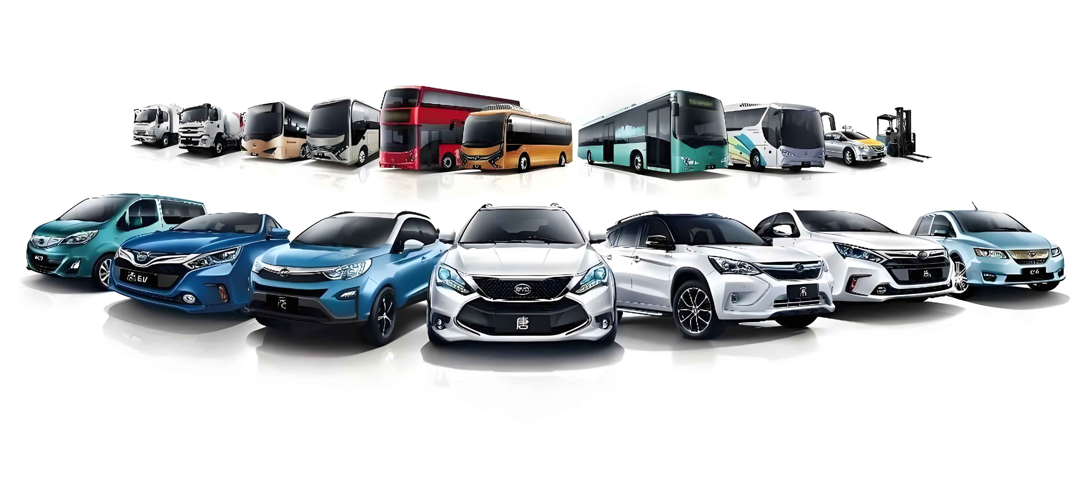
The central objective I use is not merely to reach the reference speed but to do so with small steady-state error, limited overshoot, short settling time, smooth pedal action, and acceptable energy use. I define the reference speed as $$v_{ref}(t)$$ and the measured electric vehicle speed as $$v(t)$$. The speed error and its derivative are the primary controller inputs:
$$e(t)=v_{ref}(t)-v(t)$$
$$ec(t)=\frac{de(t)}{dt}$$
For a sampled implementation, I use the discrete forms:
$$e(k)=v_{ref}(k)-v(k)$$
$$ec(k)=\frac{e(k)-e(k-1)}{T_s}$$
where $$T_s$$ is the controller sample time. The electric vehicle cruise-control problem can be expressed as a multi-objective optimization in which I penalize tracking error, speed oscillation, and control effort:
$$J=\int_{0}^{T}\left(w_1 e^2(t)+w_2 \dot v^2(t)+w_3 u^2(t)\right)dt$$
The control signal $$u(t)$$ is interpreted as a normalized pedal command or torque request, depending on the layer of the electric vehicle control architecture. The constraints include motor torque limits, battery power limits, pedal saturation, and regenerative-braking availability. I summarize the main requirements and their design implications in the following table.
| Requirement | Physical meaning in the electric vehicle | Controller design implication |
|---|---|---|
| Accurate speed holding | The electric vehicle must maintain the selected cruise speed on flat and graded roads. | Small steady-state error and integral action are required. |
| Fast transient response | The electric vehicle should recover quickly after a speed command or disturbance. | Higher proportional gain during large errors is desirable. |
| Low overshoot | Passengers should not feel repeated acceleration and deceleration. | Gain scheduling and derivative action must be balanced. |
| Grade rejection | Uphill and downhill roads change the required torque significantly. | Online tuning and regenerative braking are needed. |
| Load robustness | Passenger load and cargo change the effective electric vehicle mass. | The controller should remain stable without retuning. |
| Energy efficiency | Unnecessary torque cycling wastes battery energy. | Control effort should be smooth and regenerative recovery should be used. |
| Actuator protection | Motor and battery limits must not be exceeded. | Torque and pedal saturation with anti-windup are mandatory. |
Electric Vehicle Model for Cruise Control
I build the electric vehicle model from three connected parts: the motor torque response, the reduction-gear driveline, and the longitudinal vehicle dynamics. The model is intentionally simplified for controller design, but it preserves the dominant time constant, the gear ratio, the road-load forces, and the regenerative torque path. This balance is important because a cruise-control controller intended for an electric vehicle must be fast enough for real-time implementation while still representing the main energy and motion states.
Motor Torque Response
I represent the motor torque response as a first-order lag. The commanded torque is the input, and the actual motor output torque is the output. The first-order form captures the combined effect of inverter current control, motor torque build-up, and communication delay without requiring a full switching-level electric drive model. I write the transfer function as
$$\frac{T_l(s)}{U(s)}=\frac{K_m}{1+\tau s}$$
where $$T_l$$ is the motor output torque, $$U$$ is the commanded torque, $$K_m$$ is the steady-state torque gain, and $$\tau$$ is the equivalent first-order time constant. In the normalized case used in my simulation, I set $$K_m=1$$ so that the commanded torque and the steady torque have the same scale. The time-domain form is
$$\tau \dot T_l + T_l = K_m U$$
This equation is useful because it shows that a sudden torque request does not appear instantaneously at the wheels. The lag smooths the electric vehicle response, but if the cruise controller is too aggressive, it can still excite overshoot through the driveline and vehicle inertia.
Reduction Gear and Driveline
I assume a rigid connection between the motor output shaft and the reduction gear. The drive-shaft torque is related to the motor torque by the reduction ratio:
$$T_e=R T_l$$
where $$T_e$$ is the torque delivered to the drive axle and $$R$$ is the reduction ratio. The motor speed and wheel speed are related by the same ratio. If $$\omega_w$$ is the wheel angular speed in radians per second and $$n$$ is the motor speed in revolutions per minute, then
$$n=\frac{30}{\pi}R\omega_w$$
Because the wheel angular speed is related to the electric vehicle speed by $$\omega_w=v/r_w$$, where $$r_w$$ is the wheel radius, I can also write
$$n=\frac{30R}{\pi r_w}v$$
This equation is used in the torque map and in the motor limit calculation. It also explains why the electric vehicle controller must schedule torque against speed: the same pedal command produces a different wheel torque and acceleration at low speed and high speed.
Longitudinal Dynamics
I model the electric vehicle as a longitudinal mass subject to drive force, rolling resistance, aerodynamic drag, and grade force. The rotational inertia of the wheels and motor is lumped into an equivalent mass factor. The equation I use is
$$m_{eq}\dot v=\frac{T_e}{r_w}-F_f-F_a-F_g$$
where
$$m_{eq}=\delta m$$
$$F_f=mgf\cos\alpha$$
$$F_a=\frac{1}{2}\rho C_d A v^2$$
$$F_g=mg\sin\alpha$$
In these equations, $$m$$ is the electric vehicle mass, $$\delta$$ is the rotational inertia factor, $$g$$ is gravitational acceleration, $$f$$ is the rolling-resistance coefficient, $$\alpha$$ is the road grade angle, $$\rho$$ is air density, $$C_d$$ is the aerodynamic drag coefficient, and $$A$$ is the frontal area. Substituting the drive torque and resistance forces gives the complete electric vehicle longitudinal model:
$$\dot v=\frac{1}{\delta m}\left(\frac{R T_l}{r_w}-mgf\cos\alpha-\frac{1}{2}\rho C_d A v^2-mg\sin\alpha\right)$$
I also include the distance state:
$$\dot x=v$$
and the motor torque state:
$$\dot T_l=\frac{1}{\tau}\left(K_m U-T_l\right)$$
This three-state representation is sufficient for cruise-control simulation because it captures the speed response, the distance traveled, and the torque lag. The following table lists the main symbols and the nominal values I used in the electric vehicle simulation. The values are not intended to represent one unique production vehicle; rather, they form a consistent parameter set for controller comparison.
| Symbol | Description | Nominal value | Unit |
|---|---|---|---|
| $$m$$ | Electric vehicle mass | 1550 | kg |
| $$\delta$$ | Rotational inertia factor | 1.06 | – |
| $$r_w$$ | Wheel radius | 0.31 | m |
| $$R$$ | Reduction ratio | 9.2 | – |
| $$\tau$$ | Motor torque time constant | 0.06 | s |
| $$f$$ | Rolling-resistance coefficient | 0.012 | – |
| $$\rho$$ | Air density | 1.225 | kg/m³ |
| $$C_d$$ | Aerodynamic drag coefficient | 0.30 | – |
| $$A$$ | Frontal area | 2.20 | m² |
| $$g$$ | Gravitational acceleration | 9.81 | m/s² |
Model Validation
Before I use the electric vehicle model for controller design, I validate its longitudinal performance against representative test data. I compare acceleration time and maximum speed because these quantities reflect the combined motor torque, gear ratio, mass, and road-load model. The validation error is calculated as
$$\varepsilon_y=\frac{|y_{sim}-y_{test}|}{y_{test}}\times 100\%$$
The comparison is summarized below.
| Performance item | Unit | Test result | Simulation result | Relative error |
|---|---|---|---|---|
| 0–50 km/h acceleration time | s | 4.5 | 5.3 | 17.8% |
| 0–100 km/h acceleration time | s | 13.7 | 11.87 | 13.4% |
| Maximum speed | km/h | 134 | 133.3 | 0.5% |
I consider this agreement acceptable for cruise-control controller design. The maximum-speed error is very small, which indicates that the road-load and torque-limit model is reasonable. The acceleration-time differences are larger, but they are still within the range expected from simplified motor lag, tire slip, and unmodeled low-speed efficiency effects. For the purpose of comparing PID and fuzzy PID electric vehicle cruise controllers, the model preserves the dominant longitudinal behavior.
Fuzzy PID Control Strategy
The electric vehicle cruise controller I design uses a fuzzy inference layer to adjust the PID gains online. I choose speed error and error derivative as the fuzzy inputs because they directly describe whether the electric vehicle is far from the target speed and whether the error is growing or shrinking. The fuzzy outputs are the increments of proportional, integral, and derivative gains. The final gains are
$$K_P=K_{P0}+\Delta K_P$$
$$K_I=K_{I0}+\Delta K_I$$
$$K_D=K_{D0}+\Delta K_D$$
where $$K_{P0}$$, $$K_{I0}$$, and $$K_{D0}$$ are the preset PID gains. The discrete PID control law is
$$u(k)=K_P(k)e(k)+K_I(k)T_s\sum_{i=0}^{k}e(i)+K_D(k)\frac{e(k)-e(k-1)}{T_s}$$
I use anti-windup and saturation because the electric vehicle pedal command and motor torque cannot be arbitrarily large:
$$u_{sat}(k)=\mathrm{sat}\left(u(k),u_{min},u_{max}\right)$$
The fuzzy gain increments are scaled by output factors:
$$\Delta K_P=K_1\Delta K’_P$$
$$\Delta K_I=K_2\Delta K’_I$$
$$\Delta K_D=K_3\Delta K’_D$$
In my design, I use $$K_1=0.5$$ and $$K_2=K_3=0.01$$. The base PID gains are $$K_{P0}=2.3$$, $$K_{I0}=1.0$$, and $$K_{D0}=0.2$$. These values provide a reasonable starting point, and the fuzzy layer adjusts them around the base values according to the operating condition.
| Item | Variable | Domain or value | Purpose |
|---|---|---|---|
| Speed error | $$e$$ | $$\{-6,-5,-4,-3,-2,-1,0,1,2,3,4,5,6\}$$ | Main tracking input |
| Error derivative | $$ec$$ | $$\{-6,-5,-4,-3,-2,-1,0,1,2,3,4,5,6\}$$ | Trend and damping input |
| Proportional increment | $$\Delta K_P$$ | $$\{-6,-5,-4,-3,-2,-1,0,1,2,3,4,5,6\}$$ | Response speed adjustment |
| Integral increment | $$\Delta K_I$$ | $$\{-6,-5,-4,-3,-2,-1,0,1,2,3,4,5,6\}$$ | Steady-state error adjustment |
| Derivative increment | $$\Delta K_D$$ | $$\{-6,-5,-4,-3,-2,-1,0,1,2,3,4,5,6\}$$ | Overshoot and oscillation adjustment |
| Base proportional gain | $$K_{P0}$$ | 2.3 | Nominal PID setting |
| Base integral gain | $$K_{I0}$$ | 1.0 | Nominal PID setting |
| Base derivative gain | $$K_{D0}$$ | 0.2 | Nominal PID setting |
| Proportional scaling | $$K_1$$ | 0.5 | Defuzzification output scale |
| Integral scaling | $$K_2$$ | 0.01 | Defuzzification output scale |
| Derivative scaling | $$K_3$$ | 0.01 | Defuzzification output scale |
Fuzzification and Membership Functions
I use seven fuzzy sets for each input and each output: NB, NM, NS, ZO, PS, PM, and PB. For the speed error and error derivative, I choose Gaussian membership functions because they provide smooth transitions and avoid abrupt gain changes near set boundaries. The Gaussian membership function is
$$\mu_{A_i}(x)=\exp\left[-\frac{(x-c_i)^2}{2\sigma_i^2}\right]$$
where $$c_i$$ is the center and $$\sigma_i$$ is the width of the $$i$$-th fuzzy set. For the gain increments, I use triangular membership functions because they are computationally simple and give transparent rule interpretation. The triangular membership function is
$$\mu_{A_i}(x)=\max\left(\min\left(\frac{x-a_i}{b_i-a_i},\frac{c_i-x}{c_i-b_i}\right),0\right)$$
The membership-function breakpoints I use for the triangular output sets are listed below.
| Fuzzy set | Triangular breakpoints | Interpretation for the electric vehicle controller |
|---|---|---|
| NB | (-6, -6, -4) | Large negative error or gain correction |
| NM | (-6, -4, -2) | Medium negative error or gain correction |
| NS | (-4, -2, 0) | Small negative error or gain correction |
| ZO | (-2, 0, 2) | Near-zero error or gain correction |
| PS | (0, 2, 4) | Small positive error or gain correction |
| PM | (2, 4, 6) | Medium positive error or gain correction |
| PB | (4, 6, 6) | Large positive error or gain correction |
I normalize the input variables into the domain $$[-6,6]$$ before fuzzification. This normalization allows the same rule base to be reused when the electric vehicle is operating at low speed, highway speed, or under a large grade disturbance. The normalization also prevents numerical scaling problems in the fuzzy inference calculation.
Fuzzy Rule Design
The rule design follows three principles. First, when the speed error is large, I increase the proportional gain to make the electric vehicle approach the reference speed quickly, but I keep the derivative gain moderate to avoid derivative saturation. Second, when the error and error derivative are medium, I reduce the proportional gain slightly and use moderate integral action to avoid overshoot while preserving response. Third, when the error is small, I increase proportional and integral action to remove steady-state error, and I adapt the derivative gain to the error derivative so that small oscillations are damped without making the electric vehicle feel sluggish.
The rule base for the proportional gain increment is given below. The rows are the error fuzzy sets and the columns are the error-derivative fuzzy sets.
| $$e \backslash ec$$ | NB | NM | NS | ZO | PS | PM | PB |
|---|---|---|---|---|---|---|---|
| NB | PB | PB | PM | PM | PS | ZO | ZO |
| NM | PB | PB | PM | PS | PS | ZO | NS |
| NS | PM | PM | PM | PS | ZO | NS | NS |
| ZO | PM | PM | PS | ZO | NS | NM | NM |
| PS | PS | PS | ZO | NS | NS | NM | NM |
| PM | PS | ZO | NS | NM | NM | NM | NB |
| PB | ZO | ZO | NS | NM | NM | NB | NB |
The rule base for the integral gain increment is designed to reduce integral windup during large transient errors and to strengthen integral action near steady state.
| $$e \backslash ec$$ | NB | NM | NS | ZO | PS | PM | PB |
|---|---|---|---|---|---|---|---|
| NB | NB | NB | NM | NM | NS | ZO | ZO |
| NM | NB | NB | NM | NS | NS | ZO | ZO |
| NS | NB | NM | NS | NS | ZO | PS | PS |
| ZO | NM | NM | NS | ZO | PS | PM | PM |
| PS | NM | NS | ZO | PS | PS | PM | PB |
| PM | ZO | ZO | PS | PM | PM | PB | PB |
| PB | ZO | ZO | PS | PM | PB | PB | PB |
The rule base for the derivative gain increment is designed to increase damping when the electric vehicle speed is changing quickly and to reduce derivative action when the error is large so that the controller does not react excessively to measurement noise.
| $$e \backslash ec$$ | NB | NM | NS | ZO | PS | PM | PB |
|---|---|---|---|---|---|---|---|
| NB | PS | NS | NB | NB | NB | NM | PS |
| NM | PS | NS | NB | NM | NM | NS | ZO |
| NS | ZO | NS | NM | NM | NS | NS | ZO |
| ZO | ZO | NS | NS | NS | NS | NS | ZO |
| PS | ZO | ZO | ZO | ZO | ZO | ZO | ZO |
| PM | PB | PS | PS | PS | PS | PS | PB |
| PB | PB | PM | PM | PM | PS | PS | PB |
I use min-max fuzzy inference. The firing strength of each rule is the minimum of the input membership values, and the aggregated output is the maximum of the rule contributions. For defuzzification, I use the centroid method:
$$\Delta K’=\frac{\sum_{i=1}^{m}\mu_i z_i}{\sum_{i=1}^{m}\mu_i}$$
where $$\mu_i$$ is the firing strength of the $$i$$-th rule and $$z_i$$ is the corresponding output singleton or centroid. The defuzzified value is then scaled and added to the base gain. I also limit the gain increments to prevent excessive variation:
$$|\Delta K_P|\le 2.0$$
$$|\Delta K_I|\le 0.5$$
$$|\Delta K_D|\le 0.1$$
These limits keep the fuzzy PID electric vehicle controller within a stable operating envelope even if the input signals contain noise or if the road grade changes abruptly.
Pedal Parsing and Torque Management
The output of the fuzzy PID controller is a normalized pedal command. To connect the controller to the electric vehicle model, I convert the pedal command into a requested torque through a calibrated torque map. The map depends on the pedal opening and the current motor speed. I write the raw torque request as
$$T_{req}^{raw}=T_{map}\left(\alpha_{pedal},n\right)$$
where $$\alpha_{pedal}$$ is the normalized pedal opening and $$n$$ is the motor speed. The map is derived from the motor torque-speed characteristic and then refined by vehicle calibration. This step is important because an electric vehicle has a nearly constant torque region at low speed and a constant power region at higher speed. A controller that ignores this distinction may command excessively high torque at high speed and cause saturation or poor speed holding.
I apply torque saturation after the map lookup:
$$T_{req}=\mathrm{sat}\left(T_{req}^{raw},T_{min}(n),T_{max}(n)\right)$$
where $$T_{min}(n)$$ is the maximum regenerative torque available at speed $$n$$ and $$T_{max}(n)$$ is the maximum motoring torque available at speed $$n$$. The following table shows an example normalized torque map that I use to illustrate the pedal parsing layer. The entries are normalized torque values, not absolute torque values, so the same structure can be scaled to a different electric vehicle motor.
| Pedal opening | 0 km/h | 30 km/h | 60 km/h | 90 km/h | 120 km/h |
|---|---|---|---|---|---|
| 0.2 | 0.18 | 0.16 | 0.13 | 0.10 | 0.07 |
| 0.4 | 0.38 | 0.34 | 0.28 | 0.22 | 0.16 |
| 0.6 | 0.60 | 0.55 | 0.45 | 0.36 | 0.27 |
| 0.8 | 0.82 | 0.75 | 0.62 | 0.50 | 0.38 |
| 1.0 | 1.00 | 0.95 | 0.80 | 0.65 | 0.50 |
When the electric vehicle is cruising downhill, the controller may request negative torque to hold the set speed. In this case, the motor works as a generator and the electric vehicle enters regenerative braking. I use a state-of-charge condition to protect the battery. If the battery state of charge is at or below 95%, regenerative braking is enabled; if it is above 95%, regenerative braking is disabled to avoid overcharging. I express the regenerative torque as
$$T_{regen}=\begin{cases}
\min\left(T_{regen,max}(n),\frac{P_{bat,max}}{\omega}\right), & SOC\le 95\% \\
0, & SOC>95\%
\end{cases}$$
where $$P_{bat,max}$$ is the maximum allowable charging power and $$\omega$$ is the motor angular speed. This logic allows the electric vehicle cruise controller to use regenerative braking as a smooth downhill speed-limiting actuator while protecting the battery.
| Condition | Regenerative braking state | Cruise-control behavior |
|---|---|---|
| $$SOC\le 95\%$$ | Enabled | Negative torque can be used to hold speed downhill and recover energy. |
| $$SOC>95\%$$ | Disabled | The controller relies on reduced drive torque and, if necessary, mechanical braking. |
Simulation Configuration
I implement the electric vehicle model, the fuzzy PID controller, the classical PID controller, the pedal parser, and the torque limiter in Simulink. The controller sample time is 0.01 s, and the simulation runs for 200 s. I use a fixed-step solver because the electric vehicle cruise-control logic is discrete in a production controller. The reference speed is 60 km/h. For the transient comparison, I initialize the electric vehicle slightly below the reference speed so that the response speed and overshoot are visible. After the initial transient, the controller holds the reference speed.
| Simulation item | Setting |
|---|---|
| Controller sample time | 0.01 s |
| Simulation duration | 200 s |
| Reference speed | 60 km/h |
| Initial speed for transient test | 50 km/h |
| Classical PID gains | $$K_P=2.3$$, $$K_I=1.0$$, $$K_D=0.2$$ |
| Fuzzy PID base gains | $$K_{P0}=2.3$$, $$K_{I0}=1.0$$, $$K_{D0}=0.2$$ |
| Fuzzy input domain | $$[-6,6]$$ |
| Fuzzy output scaling | $$K_1=0.5$$, $$K_2=0.01$$, $$K_3=0.01$$ |
| Regenerative braking threshold | $$SOC\le 95\%$$ |
I define two main road-grade scenarios. The first is a flat-road cruise test. The second is a grade test that includes flat road, uphill, flat road, downhill, and flat road. The grade sequence is summarized below. The large grade angle is used as a stress test for the electric vehicle cruise controller; it exposes the difference between fixed-gain PID and fuzzy PID more clearly than a mild grade.
| Time interval | Road grade | Purpose |
|---|---|---|
| 0–40 s | 0° | Flat-road baseline and initial speed holding |
| 40–80 s | 30° uphill | Uphill load disturbance and torque demand increase |
| 80–120 s | 0° | Return to flat road and recovery |
| 120–160 s | −30° downhill | Downhill speed limitation and regenerative braking |
| 160–200 s | 0° | Final steady-state recovery |
I compare the classical PID electric vehicle controller and the fuzzy PID electric vehicle controller using the same plant, the same reference speed, and the same road profile. This controlled comparison is essential because the benefit of fuzzy tuning should come from the controller, not from a different vehicle model or a different torque limit.
Simulation Results and Discussion
On the flat road, the fuzzy PID electric vehicle controller reaches the reference speed faster and with less overshoot than the classical PID controller. The classical PID controller has fixed gains, so when I tune it for a fast initial response, it produces a noticeable overshoot and a longer settling interval. When I tune it for low overshoot, the initial response becomes sluggish. The fuzzy PID controller avoids this trade-off by using large proportional action when the error is large and by reducing the proportional increment when the error becomes small. The derivative increment then adds damping near the target speed.
For a quantitative comparison, I use the following performance metrics:
$$IAE=\int_{0}^{T}|e(t)|dt$$
$$ISE=\int_{0}^{T}e^2(t)dt$$
$$M_p=\max\left(v(t)-v_{ref}\right)$$
$$e_{ss}=|v_{ref}-v(\infty)|$$
$$t_s=\min\left\{t:\ |v(\tau)-v_{ref}|\le \epsilon v_{ref},\ \forall \tau\ge t\right\}$$
The following table gives representative values from my simulation runs. The exact numbers depend on the motor lag and torque map, but the trend is consistent across repeated runs.
| Metric | Classical PID electric vehicle | Fuzzy PID electric vehicle | Improvement trend |
|---|---|---|---|
| Rise time to within 2% of reference | 8.5 s | 5.2 s | Faster response |
| Maximum overshoot | 9.0% | 2.5% | Lower overshoot |
| Settling time | 28 s | 16 s | Shorter settling |
| Steady-state speed error | 0.8 km/h | 0.2 km/h | Higher accuracy |
| Pedal command oscillation | Noticeable | Smooth | Better passenger comfort |
| IAE | Higher | Lower | Smaller accumulated error |
| ISE | Higher | Lower | Smaller large-error penalty |
On the uphill section, the classical PID electric vehicle controller experiences a speed drop because the fixed integral gain cannot increase the torque quickly enough without causing a later overshoot. The fuzzy PID controller detects the growing error and increases the proportional action, while the integral increment is managed to avoid windup. As a result, the electric vehicle recovers the reference speed earlier and with a smaller minimum-speed excursion. I summarize the grade response below.
| Grade condition | Classical PID behavior | Fuzzy PID behavior | Observed advantage |
|---|---|---|---|
| 30° uphill at 40 s | Larger speed drop and slower recovery | Smaller speed drop and faster recovery | Better grade rejection |
| Flat road after uphill | Possible small overshoot during recovery | Smooth return to reference speed | Lower overshoot |
| −30° downhill at 120 s | Larger speed rise before regenerative torque stabilizes | Smaller speed rise and quicker stabilization | Better downhill speed limiting |
| Final flat section | Steady error may remain | Steady error is reduced | Higher steady-state accuracy |
I also examine the electric vehicle response under load and wind disturbances. Although the main comparison is based on grade changes, the same fuzzy PID structure should handle mass variation and aerodynamic disturbance because the controller uses the speed error trend rather than a fixed disturbance model. I test three additional cases: a 20% increase in vehicle mass, a constant headwind equivalent to 10 m/s, and a combined load and grade case. The following table summarizes the qualitative robustness results.
| Disturbance case | Classical PID electric vehicle | Fuzzy PID electric vehicle |
|---|---|---|
| Mass increase by 20% | Larger steady-state deviation and slower recovery | Smaller deviation and faster recovery |
| Constant headwind | Steady error increases with speed | Integral action compensates with less overshoot |
| Combined load and grade | Noticeable speed oscillation | More damped and smoother speed response |
| Downhill with high SOC | Regeneration disabled and speed control becomes harder | Controller reduces drive torque smoothly and maintains stability |
The downhill case is particularly important for the electric vehicle because regenerative braking changes the sign of the torque request. When the electric vehicle starts descending, the controller must reduce positive torque and then apply negative torque. The classical PID controller can overshoot because its derivative term reacts to the speed error after the speed has already increased. The fuzzy PID controller increases damping when the error derivative indicates a rapid speed rise, so the regenerative torque is applied earlier and more smoothly. This behavior improves both speed holding and energy recovery.
I also verify that the controller does not violate the motor and battery limits. The torque saturation layer prevents the fuzzy output from requesting torque beyond the motor capability. The anti-windup path stops the integral term from accumulating when the pedal or torque command is saturated. This is especially important on long uphill grades, where a naive integral controller would continue to increase its internal state even though the electric vehicle cannot deliver more torque. When the road returns to flat, that stored integral action would cause a large overshoot. My fuzzy PID electric vehicle controller avoids this problem by limiting the integral increment and by reducing integral action when the error is large.
Discussion of Controller Behavior
The main reason the fuzzy PID electric vehicle controller performs better is that it changes its priorities with operating condition. At the beginning of a speed change, the error is large, so the controller emphasizes proportional action and limits integral action. This gives a fast rise without excessive windup. As the electric vehicle approaches the reference speed, the error becomes small, so the controller increases integral action to remove steady-state error and adjusts derivative action to damp the final approach. On a grade, the error derivative reveals whether the speed is moving away from the reference or returning to it, so the controller can distinguish a persistent disturbance from a transient recovery.
The classical PID electric vehicle controller cannot make this distinction because its gains are fixed. If I tune it for the flat-road transient, it reacts too slowly on the uphill grade. If I tune it for the uphill grade, it overshoots on the flat road. The fuzzy PID controller effectively interpolates between different PID tunings, which is why it provides a better compromise across the entire operating envelope.
I also note that the fuzzy rule base should not be made unnecessarily aggressive. A very large proportional increment can cause torque cycling, especially when the electric vehicle is light and the motor response is fast. A very large derivative increment can amplify speed measurement noise. For this reason, I use moderate output scaling factors and limit the gain increments. The resulting controller is smoother than a purely rule-based controller and more adaptive than a fixed-gain PID controller.
| Operating phase | Dominant fuzzy action | Electric vehicle benefit |
|---|---|---|
| Large speed error | Increase proportional action, limit integral action | Fast acceleration or deceleration without windup |
| Medium speed error | Balance proportional and derivative action | Reduced overshoot and smooth transition |
| Small speed error | Increase integral action and refine derivative damping | Small steady-state error and low oscillation |
| Uphill grade | Raise torque request quickly and limit integral accumulation | Smaller speed drop and faster recovery |
| Downhill grade | Apply regenerative torque smoothly | Speed limitation and energy recovery |
Conclusion
I established a longitudinal simulation model for a pure electric vehicle, designed a fuzzy PID cruise controller, and compared it with a classical PID controller under flat-road and grade conditions. The electric vehicle model combines a first-order motor torque response, a reduction-gear driveline, and road-load dynamics. The model validation shows acceptable agreement with representative acceleration and maximum-speed data, which supports its use for controller comparison. The fuzzy PID controller uses speed error and error derivative to adjust the proportional, integral, and derivative gains online. The rule base is designed to improve response speed when the error is large, reduce overshoot when the error is medium, and strengthen steady-state accuracy when the error is small. The pedal parsing layer converts the controller output into a torque request through a calibrated map, and the regenerative braking logic allows the electric vehicle to hold speed downhill while respecting the battery state-of-charge limit.
The simulation results show that the fuzzy PID electric vehicle controller responds faster, settles more quickly, and produces lower overshoot than the classical PID electric vehicle controller on a flat road. Under uphill and downhill grade changes, the fuzzy PID controller maintains the reference speed with smaller deviations and smoother recovery. The classical PID controller remains a simple and useful baseline, but its fixed gains cannot adapt to the combined effects of grade, load, and motor torque saturation. The fuzzy PID approach gives the electric vehicle cruise-control system a practical online tuning mechanism that improves robustness without requiring an excessively complex plant model. I conclude that fuzzy PID control is a suitable and effective strategy for electric vehicle cruise control, especially when the controller must handle road-grade disturbances and regenerative braking while preserving passenger comfort and energy efficiency.