
In my work, I study how to plan charging infrastructure for the electric car in a way that is economically efficient, spatially fair, and compatible with a low-carbon power grid. The electric car has moved from a niche product to a central element of urban mobility and energy transition. Yet the growth of the electric car fleet has not been matched by an equally fast growth of charging facilities. I observe a persistent mismatch between the number of electric car users and the availability of charging points, and I also observe strong regional and temporal imbalances. In some areas, charging points are congested during peak hours, while in other areas they remain underused. This is not only a convenience problem for the electric car user; it is also a power system problem, because uncoordinated electric car charging can increase peak load, reduce voltage quality, and complicate carbon accounting. My research therefore treats the electric car as both a transport agent and a grid-connected load, and I build planning models that connect traffic demand, charging station location, charging capacity, carbon emission flow, and market interaction.
I begin from a simple premise: the electric car should not be planned for as if it were a conventional vehicle with a different fuel. The electric car interacts with the road network, the distribution network, and the carbon intensity of electricity at the same time. A charging station that is convenient for the electric car user may be expensive for the operator, and a charging price that is attractive to the electric car user may reduce the revenue of the charging point operator. At the same time, a charging station located at a low-carbon node can reduce the indirect emissions of the electric car, while a station located at a high-carbon node can increase them. I therefore formulate the planning problem as a multi-layer problem in which siting, sizing, carbon potential, and user response are considered together. The figure below illustrates the general setting of electric car charging in a coupled transport and energy environment.
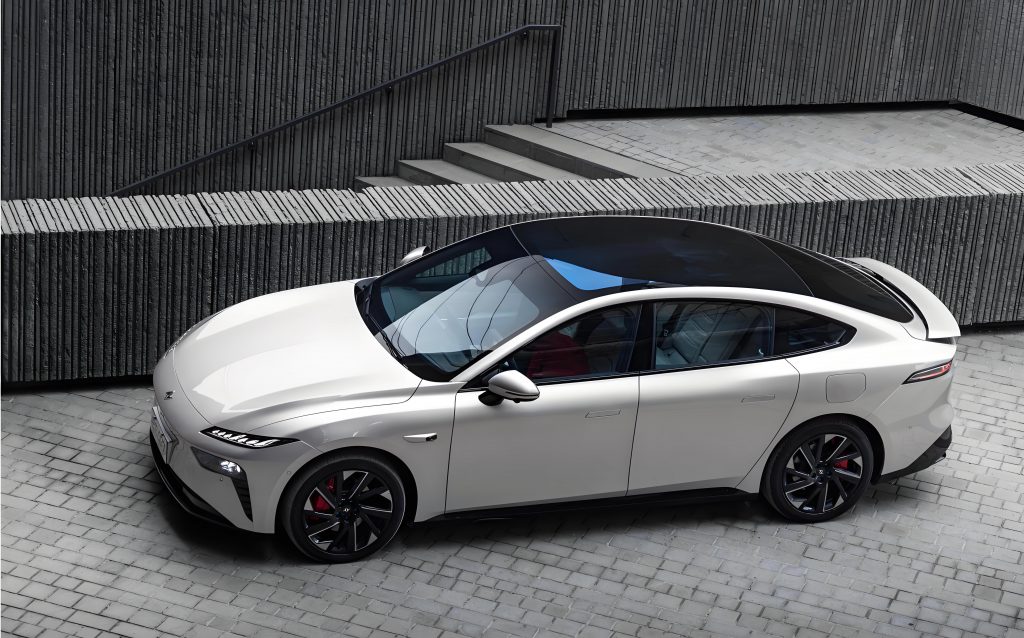
Research framing. I divide the planning problem into two connected parts. The first part focuses on plug-in charging stations for the electric car. I use a bilevel model. The upper level selects station locations with a gravity p-median model, in which each candidate station has an attraction that depends on station type, time, and node carbon potential. The lower level determines station capacity with the objective of maximizing the annual economic benefit of the charging station operator, while internalizing carbon emissions and node carbon potential. The two levels exchange location, capacity, and carbon potential. The second part extends the scope to dynamic wireless charging roads. I build a joint planning model for plug-in charging stations and dynamic wireless charging roads for the electric car, and then I add a master-slave game between the charging point operator and the electric car user. In this game, the operator sets time-of-use charging prices, and the electric car user responds with charging strategies. I use the game to examine whether the interaction can reduce user travel cost, smooth the grid load, and improve the utilization of both charging modes.
Demand forecasting for the electric car. I use Monte Carlo simulation to forecast the charging demand of the electric car. The electric car travel process is random, but it has statistical regularity. I model daily travel distance with a log-normal distribution and the start time of charging with a normal distribution that is adjusted to the 24-hour cycle. I assume that the charging power is approximately constant during the main charging period, which is a reasonable simplification for the electric car because the initial and final charging stages occupy a small share of the total charging time. I use the same battery capacity for all electric car samples in the urban case, because the case is a commuter network and long-distance diversity is not the main concern. The probability density of daily travel distance is
$$f_{D}(x)=\frac{1}{x\sigma_{D}\sqrt{2\pi}}\exp\left[-\frac{\left(\ln x-\mu_{D}\right)^{2}}{2\sigma_{D}^{2}}\right],$$
where $$\mu_{D}$$ and $$\sigma_{D}$$ are the mean and standard deviation of the logarithmic daily distance. The probability density of the charging start time is
$$f_{T}(t)=\begin{cases}
\frac{1}{\sigma_{T}\sqrt{2\pi}}\exp\left[-\frac{(t-\mu_{T})^{2}}{2\sigma_{T}^{2}}\right], & 0<t\leq &="" 12,\\[6pt]="" 12<t\leq="" 24,=""
where $$\mu_{T}$$ and $$\sigma_{T}$$ are the mean and standard deviation of the charging start time. For each electric car sample, I draw the battery capacity, the charging probability, the daily travel distance, the state of charge at the end of travel, and the charging start time. Then I calculate the charging load of the single electric car and accumulate it over the sample. When the number of samples is large enough, the load curve converges. In my simulation, I used 2000 electric car samples, with $$\mu_{D}=3.2$$, $$\sigma_{D}=0.88$$, $$\mu_{T}=17.6$$, and $$\sigma_{T}=3.4$$. The resulting load curves for residential, industrial, and commercial areas show clear differences. The industrial area has the largest total charging load, the residential area is second, and the commercial area is the smallest. The residential load peaks around 21:00, the industrial load peaks around 17:00, and the commercial load peaks around 20:00. I use these curves as the spatial and temporal input for the subsequent planning models.
Carbon emission flow and node carbon potential. I use the carbon emission flow theory to assign carbon responsibility to the electric car charging load. The carbon emission flow is a virtual flow that travels with the power flow. The branch carbon flow rate is the derivative of the branch carbon flow with respect to time, and the branch carbon flow density is the ratio of the branch carbon flow rate to the active power flow:
$$R_{l}=\frac{dF_{l}}{dt},\qquad \rho_{l}=\frac{R_{l}}{P_{l}}.$$
The node carbon potential of node $$i$$ is the weighted average carbon intensity of all power flowing into the node. I write it as
$$e_{i}=\frac{\sum_{l\in N^{+}}P_{l}\rho_{l}}{\sum_{l\in N^{+}}P_{l}},$$
where $$N^{+}$$ is the set of branches with power flowing into node $$i$$. The initial carbon potential of node $$i$$ in period $$t$$ is
$$e_{i,t}^{0}=\frac{\sum_{g\in G_{i}}P_{g,t}\mu_{g,t}+\sum_{l\in\Gamma_{i}}\phi_{l,t}P_{l,t}}{P_{L,i,t}},$$
where $$P_{g,t}$$ is the output of generator $$g$$, $$\mu_{g,t}$$ is its carbon intensity, $$\phi_{l,t}$$ is the carbon flow density of branch $$l$$, and $$P_{L,i,t}$$ is the total load at node $$i$$. This carbon potential is the basis of my low-carbon incentive mechanism. I propose a subsidy-adjusted charging price for the electric car:
$$s_{i,t}^{sd}=s_{t}^{base}-a\left(e_{i,t}-e_{a}\right)\rho,$$
where $$s_{t}^{base}$$ is the base time-of-use charging price, $$a$$ is the subsidy coefficient, $$e_{a}$$ is the average carbon potential, and $$\rho$$ is the carbon price. The government subsidy for the electric car user who chooses a low-carbon node is
$$C_{gov}=\sum_{m=1}^{N_{m}}\sum_{t=1}^{24}\sum_{i=1}^{n_{EV}}\gamma\left(e_{a}-e_{i,t}\right)P_{i,t}^{EV},$$
where $$\gamma$$ is the government subsidy carbon price and $$P_{i,t}^{EV}$$ is the charging load of station $$i$$ in period $$t$$. The actual charging cost of the electric car user is
$$C_{EV}=\begin{cases}
s_{i,t}^{sd}p_{EV}+\eta\frac{d_{i}}{v}, & Y_{ij}=0,\\[6pt]
s_{j,t}^{sd}p_{EV}+C_{gov}+\eta\frac{d_{j}}{v}, & Y_{ij}=1,
\end{cases}$$
where $$Y_{ij}$$ indicates whether the electric car user moves from station $$i$$ to station $$j$$, $$p_{EV}$$ is the planned charging energy, $$d$$ is the distance, $$v$$ is the average speed, and $$\eta$$ is the time cost. This mechanism is important in my planning model because it turns carbon potential into an economic signal that the electric car user can respond to. In other words, the electric car is not only assigned to a station by distance; it is also guided by the carbon performance of the node.
Gravity p-median siting model. I use a gravity p-median model to select charging station locations for the electric car. The traditional p-median model minimizes the demand-weighted distance to the nearest facility. It assumes that each demand point uses the nearest facility, which is not always true for the electric car. The electric car user may choose a station that is slightly farther away but more attractive, for example because it has a lower charging price, a lower carbon potential, or a better service type. The gravity p-median model captures this behavior. I define the probability that demand point $$i$$ chooses candidate station $$j$$ as
$$f_{ij}=\frac{S_{j}d_{ij}^{-\beta}}{\sum_{k\in P}S_{k}d_{ik}^{-\beta}},$$
where $$S_{j}$$ is the attraction of candidate station $$j$$, $$d_{ij}$$ is the distance, $$\beta$$ is the distance decay coefficient, and $$P$$ is the set of selected stations. I define the attraction as
$$S_{j}=k_{j}T_{t,j}\frac{a_{j}+e_{i}}{d_{ij}^{\beta}},$$
where $$k_{j}$$ is the station type coefficient, $$T_{t,j}$$ is the time coefficient, $$a_{j}$$ is the attraction coefficient, and $$e_{i}$$ is the node carbon potential. The demand allocated from $$i$$ to $$j$$ is
$$h_{ij}=D_{i}f_{ij}=D_{i}\frac{S_{j}d_{ij}^{-\beta}}{\sum_{k\in P}S_{k}d_{ik}^{-\beta}},$$
and the total travel distance objective is
$$F(P)=\sum_{i}\sum_{j\in P}h_{ij}d_{ij}=\sum_{i}\sum_{j\in P}D_{i}\frac{S_{j}d_{ij}^{1-\beta}}{\sum_{k\in P}S_{k}d_{ik}^{-\beta}}.$$
The upper-level constraints are
$$\sum_{j}X_{j}=P,\qquad \sum_{j}Y_{ij}=1,\qquad Y_{ij}\leq X_{j},\qquad X_{j},Y_{ij}\in\{0,1\},$$
where $$X_{j}$$ indicates whether candidate station $$j$$ is built, and $$Y_{ij}$$ indicates whether station $$j$$ serves demand point $$i$$. I tested the advantage of the gravity p-median model against the traditional p-median model on a simple network with eight demand points and four candidate facilities. The traditional model selected facilities F2 and F3 with an expected total cost of 92 thousand yuan, while the gravity model selected F2 and F4 with an expected total cost of 85.3 thousand yuan. The result shows that the gravity p-median model can balance distance and attraction and can produce a siting plan that is closer to actual electric car user behavior.
Bilevel plug-in charging station planning. I build a bilevel planning model for plug-in charging stations of the electric car. The upper level minimizes the total travel distance of electric car users, using the gravity p-median model described above. The lower level maximizes the annual economic benefit of the charging station operator. The lower-level objective is
$$\max F=S_{e}+S_{c}-S_{i}-S_{k}-S_{w},$$
where $$S_{e}$$ is the annual electricity sales revenue, $$S_{c}$$ is the annual low-carbon revenue, $$S_{i}$$ is the annualized construction cost, $$S_{k}$$ is the annual operation and maintenance cost, and $$S_{w}$$ is the annual waiting penalty cost. The revenue from electricity sales is
$$S_{e}=\sum_{m=1}^{N_{m}}\sum_{t=1}^{24}\sum_{i=1}^{n_{EV}}P_{i,t}^{EV}\left(s_{i,t}^{sd}-s_{t}^{w}\right),$$
where $$s_{t}^{w}$$ is the wholesale purchase price. The low-carbon revenue includes the carbon reduction revenue from the electric car and the carbon potential subsidy:
$$S_{c}=S_{c1}+S_{c2},$$
$$S_{c1}=\sum_{m=1}^{N_{m}}\sum_{t=1}^{24}\sum_{i=1}^{n_{EV}}\frac{P_{i,t}^{EV}}{M_{EV}}\delta\rho,$$
$$S_{c2}=\sum_{m=1}^{N_{m}}\sum_{t=1}^{24}\sum_{i=1}^{n_{EV}}\gamma\left(e_{a}-e_{i,t}\right)P_{i,t}^{EV},$$
where $$M_{EV}$$ is the energy consumption per 100 km, and $$\delta$$ is the carbon reduction of the electric car relative to a fuel car per 100 km. The annualized construction cost is
$$S_{i}=\sum_{i=1}^{n_{EV}}\left[s_{gd}+\frac{s_{t,EV}P_{i,EV}}{(1+d)^{q}}\right]\frac{d(1+d)^{q}}{(1+d)^{q}-1},$$
where $$s_{gd}$$ is the fixed station cost, $$s_{t,EV}$$ is the unit capacity construction cost, $$P_{i,EV}$$ is the rated capacity, $$d$$ is the discount rate, and $$q$$ is the service life. The operation and maintenance cost is
$$S_{k}=\sum_{i=1}^{n_{EV}}s_{m,EV}P_{i,EV},$$
and the waiting penalty cost is
$$S_{w}=\sum_{m=1}^{N_{m}}\sum_{t=1}^{24}\sum_{i=1}^{n_{EV}}\eta\frac{P_{i,t}^{EV}-P_{i,EV}}{P_{EV}}.$$
The constraints include total demand satisfaction, service radius coverage, capacity lower bound, branch current limit, and node voltage limit:
$$\sum_{i=1}^{n_{EV}}P_{i,EV}\geq\sum_{t=1}^{24}\sum_{i=1}^{n_{EV}}P_{i,t}^{EV},$$
$$R_{s}\leq d\left(DT_{i},DT_{i+1}\right)\leq 2R_{s},$$
$$\sum_{i=1}^{n_{EV}}P_{i,EV}\geq0.7\sum_{i=1}^{n_{EV}}\max_{t}P_{i,t}^{EV},$$
$$I_{ij}\leq I_{ij,\max},\qquad V_{i,\min}\leq V_{i}\leq V_{i,\max}.$$
I solve the bilevel model with a particle swarm algorithm for the upper level and a CPLEX solver for the lower level. The particle swarm generates candidate station locations. The lower level solves the capacity problem and returns the node carbon potential. The upper level then updates the attraction and the location. The process repeats until the carbon potential constraint is satisfied or the maximum number of iterations is reached.
Case study for plug-in charging stations. I use a 33-node traffic network coupled with an IEEE 33-node distribution system for the plug-in charging station case. The traffic network has 33 nodes and 54 urban road branches, and the nodes are divided into residential, commercial, and industrial areas. The region has 11,000 electric cars, with an energy consumption of 15 kWh per 100 km. The charging power is 10 kW. The fixed investment is 1.0 million yuan per station, the charging equipment cost is 15,000 yuan per charging gun, the annual maintenance cost is 5,000 yuan per charging gun, the service life is 20 years, and the discount rate is 0.08. The wholesale electricity price is 0.5 yuan per kWh. The carbon reduction of the electric car relative to a fuel car is 6.1 kg of CO2 per 100 km, and the carbon trading price is 0.18 yuan per kg. I set four scenarios to study the effect of the low-carbon incentive and the share of renewable generation.
Table 1. Scenario settings used in my plug-in charging station case.
| Scenario | Generation mix | Tariff | Low-carbon incentive |
|---|---|---|---|
| 1 | Thermal-dominated | Traditional time-of-use | No |
| 2 | Thermal-dominated | Traditional time-of-use | Yes |
| 3 | Renewable-dominated | High-renewable time-of-use | No |
| 4 | Renewable-dominated | High-renewable time-of-use | Yes |
The selected station nodes are 3, 13, 16, 18, 19, 20, 21, 22, 26, 29, and 31. The annual costs and revenues for the four scenarios are summarized in Table 2. In the thermal-dominated setting, the total benefit of scenario 2 is 12.71 percent higher than that of scenario 1. In the renewable-dominated setting, the total benefit of scenario 4 is 7.34 percent higher than that of scenario 3. The electricity sales revenue decreases slightly when the low-carbon incentive is introduced, but the low-carbon revenue increases enough to compensate for that decrease. The waiting penalty cost is highest in scenario 4 because the combination of time-of-use pricing and the low-carbon incentive concentrates the electric car charging demand on a smaller number of low-price and low-carbon stations.
Table 2. Annual cost and revenue of plug-in charging stations under four scenarios, in ten thousand yuan.
| Scenario | Electricity sales | Low-carbon revenue | Construction cost | Maintenance cost | Waiting penalty | Total benefit |
|---|---|---|---|---|---|---|
| 1 | 264.56 | 19.36 | 125.97 | 45.58 | 14.32 | 98.04 |
| 2 | 261.32 | 32.92 | 128.31 | 46.43 | 15.68 | 103.81 |
| 3 | 304.52 | 19.51 | 123.95 | 44.13 | 16.95 | 139.00 |
| 4 | 296.65 | 33.95 | 124.94 | 42.38 | 17.09 | 146.18 |
The total planned capacities in the four scenarios are 911.7 kW, 890.65 kW, 855.41 kW, and 758.67 kW. Scenario 1 and scenario 2 have the largest total capacity, scenario 3 is lower, and scenario 4 is the lowest. The annual construction cost and maintenance cost follow the same order. In all scenarios, the planned capacity of each station is below the peak load at that node, but the gap is not large. The reason is that the peak load at most nodes lasts for a short time. From an economic point of view, accepting a small waiting penalty is cheaper than building excessive capacity. From a service quality point of view, however, a higher capacity margin would be more desirable for the electric car user.
Table 3. Total planned capacity of plug-in charging stations under four scenarios.
| Scenario | Total planned capacity (kW) |
|---|---|
| 1 | 911.70 |
| 2 | 890.65 |
| 3 | 855.41 |
| 4 | 758.67 |
I also analyze the node carbon potential of the IEEE 33-node system. In scenario 1, the average carbon potential is about 0.52 kg per kWh. High-carbon nodes are mainly the nodes directly supplied by thermal units, such as nodes 21 and 29. Low-carbon nodes are mainly located near photovoltaic units, such as nodes 13 and 14. Between 00:00 and 07:00, the carbon potential of all nodes is similar because photovoltaic output is zero and thermal units supply the load. The carbon potential peaks during 09:00-12:00 and 15:00-20:00, which are the conventional load peak periods. In scenario 4, the average carbon potential is about 0.22 kg per kWh. The carbon potential is 57 percent lower than that in scenario 1. There are two reasons. First, the renewable share is much higher in scenario 4, so the generation-side carbon intensity is lower. Second, the low-carbon incentive guides the electric car to charge at low-carbon nodes. The average carbon potential decreases quickly in the first few iterations and then stabilizes, which shows that the electric car users respond to the carbon signal.
Grid impact. The charging load of the electric car changes the nodal voltage profile. In scenario 1, the maximum node voltage deviation is 0.085 p.u. after the charging stations are connected. In scenario 4, the maximum deviation is 0.071 p.u. This is a reduction of 16.4 percent compared with scenario 1. The largest deviation occurs around 20:00, when the electric car charging load is high. The nodes with the lowest voltage are 18 and 19, because their charging power is relatively high. The comparison shows that the low-carbon incentive not only reduces carbon emissions but also improves voltage stability. In scenario 3 and scenario 4, the high-renewable time-of-use tariff shifts the electric car charging peak to 11:00-15:00, which is away from the conventional evening peak. This reduces the peak load shock on the grid and improves the stability of the distribution system. The low-carbon incentive further performs a spatial dispatch of the electric car load: it moves charging demand from high-carbon nodes to low-carbon nodes, which reduces both the charging cost of the electric car user and the carbon intensity of the grid.
Joint planning of plug-in stations and dynamic wireless charging roads. I extend the planning problem to include dynamic wireless charging roads for the electric car. Dynamic wireless charging allows the electric car to receive energy while moving. The road embeds transmitting coils, and the electric car receives power through an onboard coil. This mode reduces the need for large onboard batteries and can shift part of the charging load from stationary stations to road segments. However, the construction cost of a dynamic wireless charging road is high, so it is not economical to deploy it everywhere. I therefore build a joint planning model that decides both the plug-in charging station locations and the dynamic wireless charging road segments. The objective is to maximize the total profit of the charging infrastructure:
$$\max C_{sa}-C_{pm}-C_{pc}-C_{inv}-C_{op},$$
where $$C_{sa}$$ is the charging revenue, $$C_{pm}$$ is the power purchase cost, $$C_{pc}$$ is the penalty cost, $$C_{inv}$$ is the construction investment, and $$C_{op}$$ is the operation cost. The revenue is
$$C_{sa}=\sum_{m=1}^{N_{m}}\left(E_{f}S_{E1,t}+E_{d}S_{E2,t}\right),$$
where $$E_{f}$$ is the plug-in charging demand, $$E_{d}$$ is the dynamic wireless charging demand, $$S_{E1,t}$$ is the plug-in charging price, and $$S_{E2,t}$$ is the wireless charging price. The power purchase cost is
$$C_{pm}=\sum_{m=1}^{N_{m}}\sum_{t=1}^{24}\sum_{l}\left(P_{de,t,l}-P_{pv,t,l}\right)S_{OG,t},$$
where $$P_{de,t,l}$$ is the charging demand power on road $$l$$, $$P_{pv,t,l}$$ is the photovoltaic output, and $$S_{OG,t}$$ is the grid purchase price. The penalty cost is
$$C_{pc}=\sum_{m=1}^{N_{m}}\beta\left(E_{f}+E_{d}-P_{g}\right),$$
where $$\beta$$ is the unit penalty and $$P_{g}$$ is the load that the operator can supply. The construction investment is
$$C_{inv}=\sum_{l}\left[S_{ta1,l}+S_{ta2,l}+\frac{S_{in1}n_{q,l}M_{1,l}+S_{in2}M_{2,l}+S_{pv}n_{pv,l}+S_{ess}n_{ess,l}}{(1+\gamma)^{\alpha}}\right],$$
where $$S_{ta1,l}$$ and $$S_{ta2,l}$$ are the initial construction costs of plug-in and wireless facilities, $$M_{1,l}$$ and $$M_{2,l}$$ are binary location decisions, $$n_{q,l}$$ is the number of charging guns, $$S_{in1}$$ and $$S_{in2}$$ are unit investment costs, $$S_{pv}$$ and $$S_{ess}$$ are photovoltaic and storage unit costs, and $$\alpha$$ is the service life. The operation cost is
$$C_{op}=\sum_{m=1}^{N_{m}}\sum_{l}\left(S_{si}n_{q,l}+S_{ro}M_{2,l}L_{l}\right)T_{u},$$
where $$S_{si}$$ and $$S_{ro}$$ are unit operation costs, $$L_{l}$$ is the road length, and $$T_{u}$$ is the number of time periods. The constraints include the number of charging facilities, the energy capacity, the price range, the power flow, the photovoltaic output, the power balance, the voltage drop, and the node voltage bounds:
$$\sum_{l}M_{1,l}\leq M_{\max1},\qquad \sum_{l}M_{2,l}\leq M_{\max2},$$
$$n_{q,l}P_{1}+n_{l,t}P_{2}\leq P_{\max,l,t},$$
$$S_{1,\min}\leq S_{E1,t}\leq S_{1,\max},\qquad S_{2,\min}\leq S_{E2,t}\leq S_{2,\max},$$
$$0\leq P_{ac,t,l}\leq M\delta\left(M_{1,l}+M_{2,l}\right),$$
$$0\leq P_{pv,t,l}\leq n_{pv,l}P_{pv,\max,l},$$
$$\sum_{w}P_{G,t,w}=P_{base,t,l}+P_{ch,t,l},$$
$$U_{t,a}-U_{t,b}=r_{w}P_{ac,t,w}+x_{w}Q_{re,t,w},$$
$$U_{\min}\leq U_{t,e}\leq U_{\max}.$$
Because the revenue term contains the product of demand and price, I use McCormick relaxation to linearize the bilinear terms. I introduce auxiliary variables $$h_{1}$$ and $$h_{2}$$ such that
$$h_{1}=E_{f}S_{E1,t},\qquad h_{2}=E_{d}S_{E2,t},$$
and the revenue is rewritten as
$$I=\sum_{m=1}^{N_{m}}\left(h_{1}+h_{2}\right).$$
The additional constraints are
$$h_{1}\geq S_{OG,t}E_{f},\qquad h_{1}\geq S_{E1,\min}E_{f}+S_{OG,t}E_{f}-S_{E1,\min}E_{f}^{\max},$$
$$h_{1}\leq S_{E1,\max}E_{f},\qquad h_{1}\leq S_{OG,t}E_{f}+S_{E1,\max}E_{f}-S_{OG,t}E_{f}^{\max},$$
and analogous constraints hold for $$h_{2}$$. For the traffic side, I use the energy demand assignment model. I do not need a detailed traffic flow pattern; I only need the energy demand assigned to each road and node. The model is
$$\min CH\left(E_{f},E_{d}\right),$$
$$\text{s.t.}\quad 0\leq E_{f}+E_{d}\leq\eta_{ep}V_{r,l}n_{r,l}E_{u},$$
$$0\leq\sum_{k}\sum_{l}\left(E_{f}+E_{d}\right)\leq E_{g}.$$
This assignment model reduces the number of variables and avoids integer traffic variables, which makes the joint planning problem easier to solve.
Joint planning case with a small network. I first use the Nguyen-Dupuis traffic network coupled with the IEEE 14-node distribution system. The traffic network has 13 nodes and 13 links, and the distribution system has 14 nodes. Each electric car has a battery capacity of 24 kWh. The cost of a dynamic wireless charging road is 10 million yuan per km, and its charging price is 3 yuan per kWh. The cost of a plug-in charging station is 30 million yuan per station, and its charging price is 1.5 yuan per kWh. Each station has 20 charging guns. I set three budget scenarios: 200 million yuan, 500 million yuan, and 900 million yuan. The planning results are shown in Table 4.
Table 4. Joint planning results under different investment budgets.
| Budget (million yuan) | Plug-in station locations | Dynamic wireless road locations |
|---|---|---|
| 200 | T1, T2, T3, T4, T7, T9 | None |
| 500 | T2, T3, T5, T12 | T10-T11, T5-T9, T6-T7 |
| 900 | T3, T5 | T8-T2, T9-T10, T10-T11, T5-T9, T6-T7 |
The ratio of plug-in stations to dynamic wireless charging roads decreases as the budget increases. With a low budget, the planner builds only plug-in stations because the fixed cost of a plug-in station is lower. With a higher budget, the planner can afford more dynamic wireless charging roads, which are more expensive but can provide charging service while the electric car is moving and can reduce waiting time. The annual costs and revenues are shown in Table 5. For the charging point operator, scenario 2 is the best choice. Its electricity sales revenue is lower than that of scenario 3, but its construction cost is also much lower. Scenario 3 builds many wireless roads and therefore has a very high construction cost. Its penalty cost is the lowest because wireless charging reduces queueing at plug-in stations. However, the high investment compresses the profit. Scenario 2 balances revenue, construction cost, and penalty cost and thus gives the highest total benefit.
Table 5. Annual cost and revenue in the small joint planning case, in ten thousand yuan.
| Scenario | Electricity sales | Power purchase | Construction | Operation | Penalty | Total benefit |
|---|---|---|---|---|---|---|
| 1 | 4,953 | 990 | 1,744 | 659 | 193 | 1,367 |
| 2 | 8,250 | 1,035 | 4,385 | 859 | 223 | 2,607 |
| 3 | 10,830 | 1,159 | 7,848 | 763 | 52 | 1,008 |
In scenario 2, the dynamic wireless charging roads are placed on T10-T11, T5-T9, and T6-T7. These links are close to the core of the traffic network and have high traffic demand. The plug-in stations are placed at nodes 2, 3, 5, and 12, which are at the edge of the traffic network. This layout is reasonable. The core links serve the electric car that travels frequently through the center, while the edge stations serve the electric car whose route does not pass through a wireless road. The two charging modes complement each other and improve the coverage of the charging network.
Joint planning case with a larger network. I then use the Sioux-Falls traffic network coupled with the IEEE 33-node distribution system. The traffic network has 24 nodes and 76 links, and the distribution system has 33 nodes. The planning result includes 7 plug-in charging stations and 8 dynamic wireless charging roads. The plug-in stations are located at T3, T8, T11, T15, T13, T20, and T23. The wireless roads are located at T1-T2, T3-T4, T11-T14, T10-T15, T15-T19, T18-T20, T2-T6, and T16-T18. In a larger network, the demand for plug-in stations is more pronounced than in the small network. This is similar to a city that has both a dense urban core and a wide suburban area. In the urban core, the traffic flow is high, so dynamic wireless charging roads can serve a large number of electric cars and generate revenue. In the suburban area, the traffic flow is lower, so plug-in stations are more economical than wireless roads. The joint planning model allocates the two charging modes according to the spatial pattern of the electric car demand.
Table 6. Joint planning result in the larger network.
| Charging mode | Locations |
|---|---|
| Plug-in charging stations | T3, T8, T11, T15, T13, T20, T23 |
| Dynamic wireless charging roads | T1-T2, T3-T4, T11-T14, T10-T15, T15-T19, T18-T20, T2-T6, T16-T18 |
Master-slave game between the operator and the electric car user. I use the planning result of the larger network as the basis for a master-slave game. The charging point operator is the leader, and the electric car user is the follower. The operator sets the time-of-use charging prices for plug-in charging and dynamic wireless charging. The electric car user then chooses the charging strategy that minimizes travel cost. The operator’s objective is
$$\max G_{1}=\sum_{t}\left(S_{cd1,t}P_{1,t}+S_{cd2,t}P_{2,t}-S_{gd,t}P_{all,t}\right),$$
where $$S_{cd1,t}$$ and $$S_{cd2,t}$$ are the prices set by the operator, $$P_{1,t}$$ and $$P_{2,t}$$ are the charging powers, and $$P_{all,t}$$ is the purchased power. The electric car user’s objective is
$$\min G_{2}=\sum_{t}\left[S_{cd1,t}P_{1,t}+S_{cd2,t}P_{2,t}+S_{w}T_{w}+S_{sh}\left(P_{1,t}+P_{2,t}\right)\right],$$
where $$S_{w}$$ is the unit waiting cost, $$T_{w}$$ is the total waiting time, and $$S_{sh}$$ is the unit depreciation cost. The constraints include the photovoltaic output, the energy storage system, the power balance, and the price bounds:
$$0\leq P_{pv,t}\leq P_{\max,t},$$
$$P_{ESS\min,t}\leq P_{ESS,t}\leq P_{ESS\max,t},\qquad 0\leq P_{ESS,in,t}\leq P_{ESS\max,t},\qquad 0\leq P_{ESS,out,t}\leq P_{ESS\max,t},$$
$$P_{sa,t}-P_{b,t}+P_{pv,t}=P_{1,t}+P_{2,t},$$
$$0\leq P_{g,t}\leq P_{g\max,t},\qquad 0\leq P_{sa,t}\leq P_{g\max,t},\qquad 0\leq P_{b,t}\leq P_{g\max,t},$$
$$S_{cd1,\min}\leq S_{cd1,t}\leq S_{cd1,\max},\qquad S_{cd2,\min}\leq S_{cd2,t}\leq S_{cd2,\max}.$$
The game has a unique equilibrium because the upper-level objective is continuous and convex in the price strategy, and the lower-level objective is a continuous convex function of the charging strategy. I solve the upper level with particle swarm optimization and the lower level with CPLEX. The particle swarm generates a time-of-use price vector for the operator. The lower level solves the electric car charging strategy for that price. The upper level updates the price according to the operator’s profit. The process continues until the maximum number of iterations is reached.
Before the game, the plug-in charging price is fixed at 1.5 yuan per kWh and the wireless charging price is fixed at 3 yuan per kWh. After the game, the plug-in price is lower for most hours. From 00:00 to 07:00, it is about 0.5 yuan per kWh. This is the valley period, and the operator’s purchase price is also low. From 08:00 onward, the price rises. The highest price is 1.35 yuan per kWh during 09:00-11:00 and 19:00-23:00. These are the peak load periods, and the operator uses the price to discourage charging during those hours. The wireless charging price also fluctuates. During 07:00-09:00 and 16:00-20:00, it is higher than the pre-game price of 3 yuan per kWh. These periods combine the conventional grid peak with the morning and evening traffic peaks, and many electric car users would use wireless charging at the same time. The higher price prevents congestion. In other periods, the wireless charging price is lower, which encourages the electric car to use wireless charging when the grid is less stressed.
Table 7. Peak-valley difference and variance of the grid load before and after the game.
| Parameter | Without game | With game | Improvement |
|---|---|---|---|
| Peak-valley difference (MW) | 119.5 | 105.2 | 11.9% |
| Variance (MW) | 34.1 | 28.9 | 15.2% |
The game reduces the peak-valley difference by 11.9 percent and the variance by 15.2 percent. This means that the time-of-use pricing and the electric car charging response smooth the grid load. The peak load decreases by up to 8.1 percent, and the valley load increases by up to 22.8 percent. The load distribution over the day becomes more balanced. This is important because a smoother load reduces the need for grid expansion and improves the utilization of renewable generation. The electric car is therefore not only a load; it also becomes a flexible resource that can respond to price signals.
Table 8. Daily travel cost of the electric car user and revenue of the charging point operator, in ten thousand yuan.
| Case | Depreciation cost | Time cost | Charging cost | Total user cost | Operator revenue |
|---|---|---|---|---|---|
| Before game | 7.32 | 17.24 | 85.29 | 109.85 | 50.94 |
| After game | 7.52 | 21.04 | 71.19 | 97.75 | 47.46 |
After the game, the charging cost of the electric car decreases by 16.5 percent, while the time cost increases by 21.9 percent. The depreciation cost increases slightly because the electric car travels a slightly longer distance to reach a cheaper or less congested charging point. The total user cost decreases by 11 percent. The operator’s revenue decreases by 6.8 percent, but the decrease is smaller than the decrease in the user’s total cost. This is the expected result of the master-slave game: the operator gives up part of the revenue to induce a charging strategy that is more efficient for the electric car user and for the grid. In my view, this is a reasonable trade-off because the charging network is a service infrastructure. A pure profit-maximizing price may be stable in the short run, but it can create queueing, congestion, and user dissatisfaction in the long run.
What I learn from the models. The first lesson is that the electric car charging station should not be planned by distance alone. The gravity p-median model shows that attraction matters. When the attraction includes carbon potential and service type, the planning result is more realistic than the traditional p-median result. The second lesson is that carbon potential can be used as an economic signal. The low-carbon incentive reduces the carbon intensity of the electric car charging load and also reduces the charging cost of the electric car user. The third lesson is that the electric car charging load can be shifted in time and space. The time-of-use price shifts the load in time, and the low-carbon incentive shifts the load in space. When the two signals are combined, the grid load becomes smoother and the carbon emissions become lower. The fourth lesson is that dynamic wireless charging is not a universal substitute for plug-in charging. The joint planning model shows that wireless roads are economically attractive in high-traffic core links, while plug-in stations remain necessary at the edge of the network. The fifth lesson is that the operator and the electric car user interact strategically. The master-slave game shows that the operator’s price and the user’s charging strategy can reach an equilibrium that reduces the user cost and improves the grid load profile, although the operator’s revenue may decrease slightly.
Model limitations and future work. I also recognize several limitations in my study. First, in the plug-in charging station planning, I do not fully integrate urban traffic planning. I do not analyze how the charging station layout affects traffic flow distribution, parking demand, or land use. This is a direction for future work because the electric car charging network is part of the urban transport system. Second, in the dynamic wireless charging model, I assume that all electric cars travel at the same speed. In reality, the electric car speed varies by road type, traffic condition, and driver behavior. The charging power of a dynamic wireless road depends on the speed and the alignment of the vehicle with the road coil. I should model this heterogeneity in future work. Third, I do not consider the possible traffic congestion caused by dynamic wireless charging roads. If many electric cars slow down to charge, the traffic flow may be affected. A more complete model should couple the traffic assignment and the wireless charging decision. Fourth, I use a deterministic carbon price and a deterministic renewable output in the planning model. In practice, carbon price and renewable generation are uncertain. A stochastic or robust planning model would be more appropriate for real-world decision-making. Fifth, I use a single operator and a single user group in the game. In reality, there may be multiple charging operators and multiple user classes with different price sensitivities and different values of time. A multi-operator game would be more realistic.
Concluding view. In my study, I treat the electric car as a coupled transport-energy agent and I build planning models that connect demand forecasting, carbon emission flow, station siting, station sizing, dynamic wireless charging, and market interaction. The plug-in charging station bilevel model shows that the gravity p-median siting model and the carbon-potential-based sizing model can improve both user convenience and operator benefit. The low-carbon incentive reduces the carbon intensity of the electric car charging load, lowers the charging cost of the electric car user, and reduces the voltage deviation of the distribution network. The joint planning model shows that plug-in stations and dynamic wireless charging roads have complementary roles. The master-slave game shows that time-of-use pricing can shift the electric car charging load, reduce the peak-valley difference, and lower the total travel cost of the electric car user. I believe that the electric car charging infrastructure should be planned as a network, not as a set of isolated stations. The electric car should be guided by both price and carbon signals, and the planning model should consider both the transport network and the power network. My results support the view that a well-designed charging network can serve the electric car user, support the charging point operator, and improve the stability and carbon performance of the power grid.