
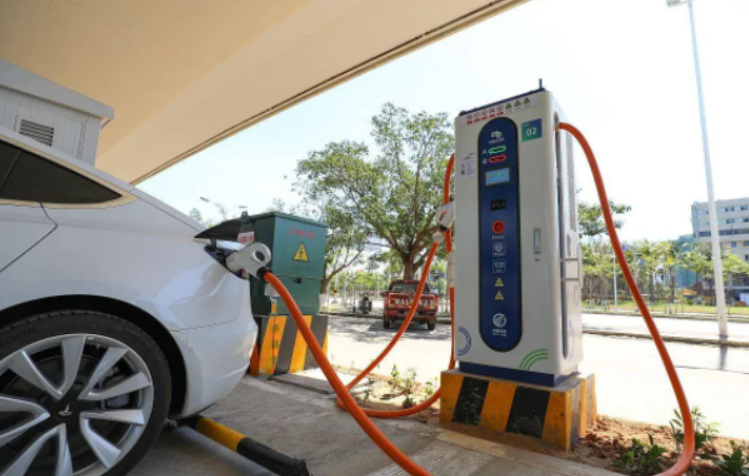
I present a practical and data-driven method for diagnosing complex faults in electric vehicle charging piles by integrating time-series representation with conventional machine learning. The motivation is straightforward: as electric vehicle charging infrastructure grows in scale and becomes more deeply embedded in daily mobility, the reliability and safety of electric vehicle charging piles directly affect user experience, maintenance cost, and public confidence. In my view, a fault diagnosis method for electric vehicle charging should not rely on a single modeling factor. Instead, it should combine maintenance work orders, historical operation bills and charging orders, and message data uploaded by the pile itself. I therefore design a diagnostic pipeline that first fuses and normalizes multi-source electric vehicle charging data, then extracts hand-crafted operational features and time-series fault representations with a bidirectional gated recurrent unit, and finally trains a machine learning classifier to determine whether a pile is faulty and, when it is faulty, which complex fault type it belongs to. The method is intended for realistic electric vehicle charging scenarios in which complex faults are rare, labels are limited, and fault symptoms are distributed across orders, messages, temperatures, voltages, and currents rather than concentrated in a single signal.
I formulate the problem as a supervised classification task over a set of electric vehicle charging pile records. Let \(\mathcal{D}=\{(x_i,y_i)\}_{i=1}^{n}\) denote the diagnostic data set, where \(x_i\) is the fused representation of the \(i\)-th pile observation and \(y_i\) is its label. For the first diagnostic task, \(y_i\in\{0,1\}\), where \(1\) indicates that the electric vehicle charging pile is faulty and \(0\) indicates that it is not faulty. For the second diagnostic task, \(y_i\in\{1,\ldots,K\}\), where \(K\) is the number of complex fault types. In my experiments, \(K=7\), covering communication faults, insulation monitoring alarms, module communication faults, charging gun overtemperature faults, battery management system communication faults, AC and DC charging faults, and data verification anomaly faults. I use the same fused representation for both tasks so that the binary decision and the multi-class fault-type decision share the same electric vehicle charging features and time-series information.
I structure the method into three cooperating layers. The first layer is multi-source data processing, which aligns work orders, charging orders, and uploaded messages. The second layer is time-series fault representation, which uses feature engineering and a bidirectional gated recurrent unit to capture both static operational evidence and dynamic electric vehicle charging behavior. The third layer is complex fault diagnosis, which trains a machine learning model on the fused representation and outputs the fault decision. This design keeps the diagnostic model interpretable while allowing the time-series model to encode subtle electric vehicle charging dynamics that are difficult to express with manual features alone.
I begin with the data sources because the quality of electric vehicle charging diagnosis depends heavily on how the evidence is aligned. A maintenance work order contains the repair request time and the recovery time. A charging order contains transaction-level information such as order count, order end reason, charging duration, current, voltage, and transaction identifiers. Uploaded messages contain the pile-side telemetry, including current, voltage, charging gun temperature, ambient temperature, and demand current. I align these sources by pile identifier and transaction serial number. For each work order, I define a pre-repair window and a post-repair window. The seven-day window immediately before the repair request is treated as a fault case, because the electric vehicle charging pile may already exhibit abnormal behavior before the user or operator reports the failure. The seven-day window immediately after recovery is treated as a non-fault case, because the pile is expected to have returned to normal operation. This windowing strategy is important for electric vehicle charging diagnosis because it connects maintenance records to actual charging behavior rather than relying only on the work-order text.
I define the multi-source observation as \(X_i=\{W_i,O_i,M_i\}\), where \(W_i\) is the work-order record, \(O_i\) is the set of charging orders in the window, and \(M_i\) is the set of uploaded messages linked to those orders. The diagnostic label is associated with the window, not with an isolated message. I then construct a fused feature vector \(x_i\) that contains both manual features and time-series representations. The overall fused representation is
$$x_i=\left[v_i^{\mathrm{manual}};v_i^{\mathrm{time}}\right],$$
where \(v_i^{\mathrm{manual}}\in\mathbb{R}^{m}\) is the engineered feature vector and \(v_i^{\mathrm{time}}\in\mathbb{R}^{d}\) is the learned time-series representation. In my implementation, \(m=119\) and \(d=32\). The dimensionality of the manual feature vector is larger because it includes one-hot encodings, daily order ratios, invalid-order ratios, temperature statistics, and current-related indicators. The time-series representation is deliberately compact so that it can be concatenated with the manual features without dominating the classifier.
I summarize the main notation in Table 1. The notation is used consistently across feature construction, sequence encoding, model training, and evaluation.
Table 1. Notation used in my electric vehicle charging fault diagnosis method.
| Symbol | Meaning |
|---|---|
| \(\mathcal{D}\) | Diagnostic data set of electric vehicle charging pile observations |
| \(n\) | Number of observations |
| \(x_i\) | Fused representation of the \(i\)-th observation |
| \(y_i\) | Fault label or fault-type label |
| \(K\) | Number of complex fault types |
| \(W_i\) | Work-order record associated with the \(i\)-th observation |
| \(O_i\) | Charging orders in the observation window |
| \(M_i\) | Uploaded message records linked to the orders |
| \(T_{\mathrm{repair}}\) | Repair request time in the work order |
| \(T_{\mathrm{fix}}\) | Recovery time in the work order |
| \(v_i^{\mathrm{manual}}\) | Engineered feature vector |
| \(v_i^{\mathrm{time}}\) | Learned time-series representation |
| \(m\) | Dimension of the manual feature vector |
| \(d\) | Dimension of the time-series representation |
| \(L\) | Length of an aligned electric vehicle charging sequence |
| \(\theta\) | Parameters of the machine learning classifier |
| \(\Theta\) | Trainable parameters of the diagnostic model |
| \(\lambda\) | Regularization balance coefficient |
I select features that are operationally meaningful for electric vehicle charging piles. The first group concerns order termination and order volume. The fault order end reason is important because abnormal termination is often the earliest observable symptom of an electric vehicle charging fault. I define 44 different order end reasons and encode each reason with a 97-dimensional one-hot vector. The encoding is
$$e_k=[0,\ldots,0,1,0,\ldots,0]\in\{0,1\}^{97},\quad e_k(k)=1,$$
where \(k\in\{0,\ldots,43\}\) is the index of the order end reason. The one-hot encoding avoids imposing an artificial ordinal relationship among end reasons, which is appropriate for electric vehicle charging diagnosis because a communication interruption and a gun overtemperature event are qualitatively different failure modes rather than ordered severity levels.
I also use total order count, fault order count, invalid order count, daily order ratios, daily fault-order ratios, daily invalid-order ratios, last-day order ratio, relative gap between demand current and actual current, average current of two consecutive orders, charging gun temperature, and ambient temperature. These features reflect both the operational load of the pile and the physical behavior of the electric vehicle charging process. For example, a sudden drop in total orders may indicate that users are avoiding a faulty pile, while an increase in invalid orders with durations below one minute may indicate repeated connection failures. A small relative gap between demand current and actual current can indicate that the pile is unable to deliver the requested current, which is a meaningful signal in electric vehicle charging diagnosis. Consecutive low average current can also indicate a module-level or connector-level problem. Charging gun temperature and ambient temperature provide context for overtemperature faults, especially during high-power electric vehicle charging in hot weather.
Table 2. Engineered features used in my electric vehicle charging pile diagnosis.
| Feature group | Feature description | Diagnostic interpretation |
|---|---|---|
| Order end reason | One-hot encoding of 44 fault order end reasons | Captures abnormal termination patterns in electric vehicle charging orders |
| Total order count | Number of charging orders in the window | Reflects pile utilization and user avoidance behavior |
| Fault order count | Number of fault orders in the window | Measures the concentration of abnormal electric vehicle charging events |
| Invalid order count | Number of orders with duration below one minute | Indicates connection failure, handshake failure, or early termination |
| Daily order ratio | Order count on each of seven days divided by total orders | Captures temporal changes in electric vehicle charging demand |
| Daily fault-order ratio | Fault orders on each day divided by daily orders | Captures the evolution of fault symptoms over time |
| Daily invalid-order ratio | Invalid orders on each day divided by daily orders | Captures repeated short failures in electric vehicle charging |
| Last-day order ratio | Order ratio on the last day of the window | Separates pre-repair degradation from post-repair recovery |
| Relative current gap | Absolute difference between demand current and actual current divided by demand current | Detects current delivery deficiency in electric vehicle charging |
| Consecutive average current | Average current of two consecutive orders | Detects persistent low-current behavior |
| Charging gun temperature | Temperature measured at the charging gun | Supports overtemperature and connector fault diagnosis |
| Ambient temperature | Historical weather temperature | Provides environmental context for thermal electric vehicle charging faults |
I normalize the features to reduce scale effects. For the total order count, I use the normalization form
$$M’_{t,j}=\frac{M_{t,j}}{M_{t,\max}-M_{t,j}},$$
where \(M_{t,j}\) is the total order count of the \(j\)-th sample and \(M_{t,\max}\) is the maximum total order count in the data set. For daily order counts, I use a ratio normalization:
$$M’_{i,j}=\frac{M_{i,j}}{\sum_{i=1}^{7}M_{i,j}},$$
where \(M_{i,j}\) is the order count on the \(i\)-th day for the \(j\)-th sample. These transformations preserve the relative electric vehicle charging activity while preventing features with large raw magnitudes from dominating the classifier. For continuous physical variables such as current, voltage, and temperature, I apply min-max scaling within each sequence so that the time-series encoder receives values in a stable range:
$$\tilde{s}_{t,k}=\frac{s_{t,k}-\min_{t}s_{t,k}}{\max_{t}s_{t,k}-\min_{t}s_{t,k}+\epsilon},$$
where \(\epsilon\) is a small positive constant used to avoid division by zero. This step is important because voltage, current, and temperature have different units and different dynamic ranges in electric vehicle charging data.
I now describe the time-series fault representation layer. After sorting historical charging orders by pile identifier and time, I link each order to its uploaded messages through the transaction serial number. I then align current, voltage, charging gun temperature, ambient temperature, demand current, and current gap at the message timestamps. The resulting sequence for the \(j\)-th observation is
$$S_j=\{s_{j,1},s_{j,2},\ldots,s_{j,L}\},$$
where \(s_{j,t}\in\mathbb{R}^{p}\) is the feature vector at time step \(t\), \(L\) is the sequence length, and \(p\) is the number of time-varying channels. I use the aligned sequence to capture the dynamics of electric vehicle charging, because many complex faults do not appear as a single abnormal value but as a pattern of drift, oscillation, repeated dropouts, or thermal rise over time.
I choose a bidirectional gated recurrent unit because it can capture both forward and backward temporal dependencies while using fewer parameters than a comparable long short-term memory network. This parameter efficiency matters in my setting because complex fault samples are rare. A large model can easily overfit the limited number of complex electric vehicle charging fault cases. The gated recurrent unit uses an update gate and a reset gate to control information flow. For the forward direction, I write
$$z_t^{(f)}=\sigma\left(W_{zx}s_t+U_{zh}h_{t-1}^{(f)}+b_z\right),$$
$$r_t^{(f)}=\sigma\left(W_{rx}s_t+U_{rh}h_{t-1}^{(f)}+b_r\right),$$
$$\tilde{h}_t^{(f)}=\tanh\left(W_{hx}s_t+U_h\left(r_t^{(f)}\odot h_{t-1}^{(f)}\right)+b_h\right),$$
$$h_t^{(f)}=\left(1-z_t^{(f)}\right)\odot h_{t-1}^{(f)}+z_t^{(f)}\odot\tilde{h}_t^{(f)}.$$
For the backward direction, I use
$$z_t^{(b)}=\sigma\left(W_{zx}s_t+U_{zh}h_{t+1}^{(b)}+b_z\right),$$
$$r_t^{(b)}=\sigma\left(W_{rx}s_t+U_{rh}h_{t+1}^{(b)}+b_r\right),$$
$$\tilde{h}_t^{(b)}=\tanh\left(W_{hx}s_t+U_h\left(r_t^{(b)}\odot h_{t+1}^{(b)}\right)+b_h\right),$$
$$h_t^{(b)}=\left(1-z_t^{(b)}\right)\odot h_{t+1}^{(b)}+z_t^{(b)}\odot\tilde{h}_t^{(b)}.$$
The forward and backward hidden states are concatenated at each time step:
$$h_t=\left[h_t^{(f)};h_t^{(b)}\right].$$
I use the final concatenated hidden state or a pooled version of the sequence as the time-series representation:
$$v_i^{\mathrm{time}}=\mathrm{Pool}\left(\left\{h_1,h_2,\ldots,h_L\right\}\right).$$
In my implementation, I use the last hidden state of the bidirectional encoder after mean pooling over the sequence. The representation is then concatenated with the manual feature vector:
$$v_i^{\mathrm{merge}}=\left[v_i^{\mathrm{manual}};v_i^{\mathrm{time}}\right].$$
I summarize the time-series channels in Table 3. These channels are the physical and operational signals that carry the strongest electric vehicle charging fault evidence in my data.
Table 3. Time-series channels used by the bidirectional gated recurrent unit.
| Channel | Variable | Role in electric vehicle charging diagnosis |
|---|---|---|
| Voltage | \(V_t\) | Detects abnormal voltage regulation and module-level faults |
| Current | \(I_t\) | Detects current delivery deficiency and interruption patterns |
| Demand current | \(I_t^{\mathrm{dem}}\) | Provides the requested current baseline for comparison |
| Current gap | \(I_t^{\mathrm{dem}}-I_t\) | Measures the mismatch between request and delivery |
| Charging gun temperature | \(T_t^{\mathrm{gun}}\) | Captures connector heating and overtemperature risk |
| Ambient temperature | \(T_t^{\mathrm{amb}}\) | Provides environmental context for thermal behavior |
| Order state | \(q_t\) | Encodes charging, stopping, fault, and idle states |
| Time index | \(t\) | Preserves the temporal order of electric vehicle charging events |
I train the time-series encoder and the classifier in a coordinated way. The classifier receives the fused representation and minimizes a regularized empirical loss:
$$\theta^*=\arg\min_{\Theta}\frac{1}{n}\sum_{i=1}^{n}L\left(f_\theta\left(v_i^{\mathrm{merge}}\right),y_i\right)+\lambda\Omega(\Theta),$$
where \(f_\theta\) is the classifier, \(L\) is the task loss, \(\Omega(\Theta)\) is a regularization term, and \(\lambda\) balances fit and complexity. For the binary task, I use the binary cross-entropy loss:
$$L_{\mathrm{BCE}}=-\left[y\log\hat{p}+(1-y)\log(1-\hat{p})\right],$$
where \(\hat{p}\) is the predicted probability that the electric vehicle charging pile is faulty. For the multi-class task, I use the categorical cross-entropy loss:
$$L_{\mathrm{CE}}=-\sum_{k=1}^{K}y_k\log\hat{y}_k,$$
where \(y_k\) is the one-hot fault-type label and \(\hat{y}_k\) is the predicted probability of fault type \(k\). I set the decision threshold to 0.5 for the binary task. If the predicted fault probability is greater than the threshold, I classify the pile as faulty; otherwise, I classify it as normal.
I face a severe class imbalance problem. After cleaning and aligning the electric vehicle charging data, the number of complex fault samples is small. In my data set, the original set contains 138 observations, with 70 faulty observations and 68 non-faulty observations. The number of samples for each complex fault type is much smaller than the number of normal electric vehicle charging observations. To mitigate this issue, I apply the synthetic minority oversampling technique to the minority fault types. The method generates synthetic samples by interpolating between a minority sample and one of its nearest minority neighbors:
$$x_{\mathrm{new}}=x_i+\gamma\left(x_{ij}-x_i\right),$$
where \(x_i\) is a minority sample, \(x_{ij}\) is a randomly selected nearest neighbor from the same minority class, and \(\gamma\in[0,1]\) controls the interpolation position. I use two nearest neighbors within the same class and generate synthetic samples at approximately three times the original minority count for the small fault types. I prefer this interpolation approach over simple duplication because duplication can amplify the same electric vehicle charging pattern and increase overfitting, whereas interpolation creates modest variations in the feature space and improves the classifier’s ability to generalize across similar complex faults.
I build two diagnostic tasks from the same fused representation. Task 1 is a binary task that decides whether an electric vehicle charging pile is faulty. Task 2 is a multi-class task that decides the complex fault type among seven categories. The training and test partitions are manually controlled because the sample size is small and the time order of electric vehicle charging observations matters. I use approximately an 80/20 split, resulting in 165 training observations and 51 test observations after augmentation. The detailed composition is shown in Table 4.
Table 4. Diagnostic tasks and data composition after minority augmentation.
| Diagnostic task | Class | Training count | Test count |
|---|---|---|---|
| Task 1: faulty or not | Faulty | 108 | 40 |
| Task 1: faulty or not | Non-faulty | 57 | 11 |
| Task 2: fault type | Communication fault | 14 | 5 |
| Task 2: fault type | Insulation monitoring alarm | 10 | 6 |
| Task 2: fault type | Module communication fault | 10 | 5 |
| Task 2: fault type | Charging gun overtemperature | 19 | 6 |
| Task 2: fault type | Battery management system communication fault | 20 | 6 |
| Task 2: fault type | AC and DC charging fault | 16 | 6 |
| Task 2: fault type | Data verification anomaly | 19 | 6 |
| Task 2: fault type | No fault | 57 | 11 |
I evaluate the diagnostic performance with accuracy, precision, recall, and the F1 value. These metrics are computed from the confusion-matrix counts:
$$\mathrm{Accuracy}=\frac{TP+TN}{TP+TN+FP+FN}\times 100\%,$$
$$\mathrm{Precision}=\frac{TP}{TP+FP}\times 100\%,$$
$$\mathrm{Recall}=\frac{TP}{TP+FN}\times 100\%,$$
$$F_1=2\times\frac{\mathrm{Precision}\times\mathrm{Recall}}{\mathrm{Precision}+\mathrm{Recall}}\times 100\%.$$
Here, \(TP\) is the number of faulty electric vehicle charging observations correctly identified as faulty, \(TN\) is the number of non-faulty observations correctly identified as non-faulty, \(FP\) is the number of non-faulty observations incorrectly identified as faulty, and \(FN\) is the number of faulty observations incorrectly identified as non-faulty. For the multi-class task, I compute the same metrics in a one-versus-rest manner and average them across classes.
I first compare my fused representation against conventional classifiers trained only on manual features. I use decision tree, random forest, neural network, AdaBoost, and naive Bayes classifiers. I keep the training and test partitions identical across methods so that the comparison isolates the effect of the time-series representation. Table 5 reports the results for Task 1. The fused representation improves most of the classifiers, and the decision tree benefits consistently. The decision tree with the bidirectional gated recurrent unit representation reaches 96.09 percent accuracy and 95.76 percent F1, which is a clear improvement over the decision tree trained on manual features alone. I interpret this result as evidence that the time-series representation adds complementary information about electric vehicle charging dynamics that the manual order-level features do not capture.
Table 5. Task 1 results for faulty versus non-faulty electric vehicle charging piles.
| Model | Accuracy (%) | Precision (%) | Recall (%) | F1 (%) |
|---|---|---|---|---|
| Decision Tree | 84.32 | 87.87 | 84.32 | 86.04 |
| Random Forest | 84.32 | 85.56 | 84.32 | 84.94 |
| Neural Network | 96.09 | 96.27 | 96.09 | 96.18 |
| AdaBoost | 86.27 | 87.42 | 86.27 | 86.86 |
| Naive Bayes | 92.16 | 92.46 | 92.16 | 92.32 |
| Bi-GRU representation + Decision Tree | 96.09 | 95.63 | 96.09 | 95.76 |
| Bi-GRU representation + Random Forest | 92.16 | 92.55 | 92.16 | 92.44 |
| Bi-GRU representation + Neural Network | 96.09 | 96.27 | 96.09 | 96.18 |
| Bi-GRU representation + AdaBoost | 94.12 | 95.23 | 94.12 | 94.68 |
| Bi-GRU representation + Naive Bayes | 92.16 | 92.46 | 92.16 | 92.32 |
For Task 2, the multi-class fault-type diagnosis is harder because several complex fault types share similar electric vehicle charging symptoms. Table 6 shows that the fused representation improves the decision tree substantially. The decision tree with the bidirectional gated recurrent unit representation reaches 60.78 percent accuracy and 63.98 percent F1. This result is not perfect, but it is meaningful in a small-sample electric vehicle charging diagnosis setting where the classes are highly imbalanced and several fault types have overlapping signatures. The improvement in precision is especially important because false alarms increase maintenance cost and reduce trust in electric vehicle charging infrastructure.
Table 6. Task 2 results for complex fault-type diagnosis of electric vehicle charging piles.
| Model | Accuracy (%) | Precision (%) | Recall (%) | F1 (%) |
|---|---|---|---|---|
| Decision Tree | 49.02 | 62.42 | 49.02 | 54.92 |
| Random Forest | 50.10 | 29.13 | 50.10 | 36.86 |
| Neural Network | 54.90 | 56.32 | 54.90 | 55.60 |
| AdaBoost | 52.94 | 55.12 | 52.94 | 53.92 |
| Naive Bayes | 56.86 | 43.12 | 56.86 | 49.12 |
| Bi-GRU representation + Decision Tree | 60.78 | 67.56 | 60.78 | 63.98 |
| Bi-GRU representation + Random Forest | 52.94 | 29.79 | 52.94 | 38.14 |
| Bi-GRU representation + Neural Network | 54.90 | 56.32 | 54.90 | 55.60 |
| Bi-GRU representation + AdaBoost | 58.82 | 62.14 | 58.82 | 60.54 |
| Bi-GRU representation + Naive Bayes | 56.86 | 43.12 | 56.86 | 49.12 |
I then compare different time-series encoders while keeping the classifier fixed as a decision tree. The purpose of this comparison is to determine whether the bidirectional gated recurrent unit is actually necessary for electric vehicle charging fault representation or whether a simpler recurrent model would suffice. I evaluate a plain recurrent neural network, a long short-term memory network, a gated recurrent unit, a bidirectional long short-term memory network, and the bidirectional gated recurrent unit. All models use the same hidden dimension, layer count, and dropout rate. The results are reported in Table 7.
Table 7. Comparison of time-series encoders with a decision tree classifier.
| Task | Encoder | Accuracy (%) | Precision (%) | Recall (%) | F1 (%) |
|---|---|---|---|---|---|
| Task 1 | None | 84.32 | 87.87 | 84.32 | 86.04 |
| Task 1 | RNN | 88.24 | 90.48 | 88.24 | 89.36 |
| Task 1 | LSTM | 88.57 | 90.75 | 88.57 | 89.64 |
| Task 1 | GRU | 92.86 | 93.75 | 92.86 | 93.30 |
| Task 1 | Bi-LSTM | 94.29 | 94.89 | 94.29 | 94.56 |
| Task 1 | Bi-GRU | 96.09 | 95.63 | 96.09 | 95.76 |
| Task 2 | None | 49.02 | 62.42 | 49.02 | 54.92 |
| Task 2 | RNN | 53.57 | 66.07 | 53.57 | 59.14 |
| Task 2 | LSTM | 53.57 | 66.96 | 53.57 | 59.48 |
| Task 2 | GRU | 53.57 | 68.45 | 53.57 | 60.08 |
| Task 2 | Bi-LSTM | 57.14 | 62.76 | 57.14 | 59.82 |
| Task 2 | Bi-GRU | 60.78 | 67.56 | 60.78 | 63.98 |
I observe that all time-series encoders improve over the decision tree without time-series representation, which confirms that temporal electric vehicle charging behavior is informative. The bidirectional models outperform their unidirectional counterparts in most settings, and the bidirectional gated recurrent unit gives the best overall balance. I attribute this to two factors. First, the bidirectional structure sees both the pre-fault evolution and the post-event recovery pattern, which is useful when the fault symptom is a transient event surrounded by normal electric vehicle charging behavior. Second, the gated recurrent unit has fewer parameters than the long short-term memory network, which reduces overfitting on the small complex fault sample set. In my electric vehicle charging diagnosis task, a smaller and more regularized recurrent encoder is preferable to a larger model that memorizes the scarce fault cases.
I tune the hidden dimension of the bidirectional gated recurrent unit. I compare 16, 32, and 64 dimensions under the same training configuration. A dimension of 32 gives the best accuracy for both diagnostic tasks. A dimension of 16 underfits the temporal electric vehicle charging patterns, while a dimension of 64 increases the risk of overfitting and does not improve the test performance. I therefore use 32 as the representation dimension. The main hyperparameters are summarized in Table 8.
Table 8. Selected hyperparameters for the time-series representation and classifier.
| Parameter | Search or candidate values | Selected value | Reason |
|---|---|---|---|
| Bi-GRU hidden dimension | 16, 32, 64 | 32 | Best balance between underfitting and overfitting |
| Number of Bi-GRU layers | 2, 4, 6 | 6 | Captures multi-scale electric vehicle charging dynamics |
| Dropout rate | 0.1, 0.2, 0.3 | 0.3 | Regularizes the small-sample recurrent encoder |
| Optimizer | Adam | Adam | Stable convergence on sparse electric vehicle charging data |
| Learning rate | 0.0001, 0.001, 0.01 | 0.001 | Fast enough without unstable updates |
| Regularization coefficient \(\lambda\) | 0.001, 0.01, 0.1 | 0.01 | Prevents overfitting while preserving fault sensitivity |
| Decision threshold | 0.5 | 0.5 | Standard threshold for binary electric vehicle charging fault diagnosis |
I also examine the effect of the time-series representation dimension on the decision tree. Table 9 summarizes my observations from the dimension comparison. The exact ranking is task-dependent, but the 32-dimensional representation is consistently the best choice in my experiments. The result supports a design principle for electric vehicle charging fault diagnosis: the time-series representation should be compact enough to avoid overfitting but expressive enough to encode voltage, current, temperature, and order-state dynamics.
Table 9. Dimension comparison for the bidirectional gated recurrent unit representation.
| Dimension | Observed behavior | Decision |
|---|---|---|
| 16 | Insufficient capacity for multi-channel electric vehicle charging dynamics | Not selected |
| 32 | Best accuracy and F1 for both diagnostic tasks | Selected |
| 64 | Higher overfitting risk with scarce complex fault samples | Not selected |
I further analyze why the fused representation works. The manual features encode order-level evidence such as failure frequency, invalid orders, daily trends, current deficiency, and temperature. These features are useful but coarse. The recurrent representation encodes the order of events and the shape of the electric vehicle charging trajectory. For example, a communication fault may appear as repeated short orders and missing message segments, whereas an overtemperature fault may appear as a gradual rise in gun temperature under high current. A module communication fault may appear as current oscillation or a sudden drop in delivered current. A data verification anomaly may produce inconsistent order end reasons without a strong thermal signature. The fused representation allows the classifier to combine the order-level statistics with the temporal shape of these electric vehicle charging symptoms.
I also find that the bidirectional representation improves the diagnosis of faults that occur near the boundary of the observation window. In many electric vehicle charging cases, the first abnormal order is followed by a few normal orders because the pile recovers temporarily or because different users use different charging parameters. A unidirectional encoder may overemphasize the most recent normal behavior, while a bidirectional encoder can use the later recovery context and the earlier fault onset jointly. This is especially useful when the work-order time is not perfectly aligned with the actual fault onset. The bidirectional representation is therefore not merely a modeling choice; it matches the retrospective nature of maintenance-driven electric vehicle charging fault diagnosis.
I take several steps to avoid data leakage. First, I split by observation window rather than by individual message. If messages from the same electric vehicle charging order appeared in both training and test sets, the evaluation would be overly optimistic. Second, I apply minority augmentation only to the training set. The test set remains unchanged so that the reported metrics reflect performance on original electric vehicle charging observations. Third, I fix the classifier and encoder settings before the final test evaluation. I do not tune on the test set. These controls are important because the data set is small and complex fault types are rare.
I compare my method with single-model baselines in Table 10. The table summarizes the main takeaway rather than repeating every metric. The fused method is more consistent across the two tasks. A standalone decision tree is interpretable but misses temporal electric vehicle charging evidence. A standalone neural network can fit nonlinear patterns but is less stable when complex fault samples are scarce. The fused representation with a decision tree provides a good compromise between accuracy, interpretability, and robustness.
Table 10. Summary comparison of diagnostic strategies for electric vehicle charging piles.
| Strategy | Strength | Limitation | Observed outcome |
|---|---|---|---|
| Manual features only | Interpretable and fast | Ignores temporal electric vehicle charging dynamics | Lower accuracy and F1, especially for complex fault types |
| Deep sequence model only | Captures temporal patterns | Needs more data and is harder to interpret | Good potential but unstable with scarce complex faults |
| Fused manual and Bi-GRU representation | Combines order-level and temporal evidence | Requires careful alignment and normalization | Best overall accuracy, precision, recall, and F1 in my experiments |
I discuss the operational implications for electric vehicle charging infrastructure. A diagnosis method that uses work orders, historical orders, and uploaded messages can be integrated into an electric vehicle charging operation center. The center can monitor order termination reasons, invalid order ratios, current delivery gaps, and gun temperature trends. When the binary classifier raises a fault alarm, the multi-class classifier can provide a probable fault type and guide the dispatch of maintenance resources. This is valuable because different complex faults require different responses. A communication fault may be addressed by a software reset or network check, while an overtemperature fault may require inspection of the connector and cooling path. A module communication fault may require replacement of a power module. A data verification anomaly may require checking the meter, communication gateway, or encryption configuration. By mapping the predicted fault type to a maintenance procedure, the method can reduce downtime and improve the user experience of electric vehicle charging.
I also consider the limitations. The first limitation is sample size. Complex faults in electric vehicle charging piles are rare, and the number of labeled cases is small. Although minority augmentation helps, synthetic samples cannot replace real complex fault cases. The second limitation is label noise. A work order may be opened for a symptom that is not directly caused by the pile, and the repair record may not fully describe the root cause. The third limitation is concept drift. Electric vehicle charging hardware, firmware, and user behavior change over time, so a model trained on one period may need recalibration. The fourth limitation is that the current representation uses order and message data but does not explicitly model the internal power-electronics topology of the charger. A hybrid approach that combines data-driven electric vehicle charging diagnosis with physical models could improve interpretability and transferability.
I propose several directions for future work. I plan to introduce pretraining on unlabeled electric vehicle charging message sequences so that the recurrent encoder can learn general temporal patterns before fine-tuning on scarce fault labels. I also plan to explore few-shot learning and metric learning for complex fault types with very few examples. Another direction is to incorporate attention mechanisms that can highlight which time steps and channels contribute most to a fault decision. This would make the diagnosis more transparent for maintenance engineers. I also intend to evaluate the method across multiple cities and multiple charger models to test its robustness under domain shift. Finally, I plan to study cost-sensitive learning because the cost of a missed electric vehicle charging fault is not equal to the cost of a false alarm. A missed overtemperature fault can create a safety risk, while a false alarm increases inspection workload. A cost-sensitive decision threshold could better align the diagnostic model with operational priorities.
In summary, I have described a method that integrates time-series representation into complex fault diagnosis for electric vehicle charging piles. The method fuses work orders, historical orders, and uploaded messages, normalizes heterogeneous features, encodes electric vehicle charging dynamics with a bidirectional gated recurrent unit, and trains a machine learning classifier on the fused representation. In my experiments, the method improves accuracy, precision, recall, and F1 over manual-feature baselines and over several recurrent encoders. The bidirectional gated recurrent unit is particularly suitable for small-sample electric vehicle charging fault diagnosis because it captures both forward and backward temporal context while keeping the parameter count manageable. I believe that time-series-aware electric vehicle charging fault diagnosis is a practical path toward safer, more reliable, and more maintainable electric vehicle charging infrastructure.