
I have spent a considerable part of my engineering practice on the reliability of the electric vehicle battery pack, and the longer I work with real fleets the more convinced I become that the dominant bottleneck is not the chemistry of the cells but the way we diagnose and schedule maintenance around them. An electric vehicle battery pack is a complex, multi-domain system in which electrochemical, thermal, electrical, and mechanical processes are coupled together and evolve continuously during operation. When a cell begins to drift, when a module begins to heat unevenly, or when internal resistance starts to climb, the symptoms are subtle and they appear long before a driver notices anything. Traditional diagnostic routines, which I have used and audited in workshops, rely on single-parameter thresholds or static bench measurements, and they systematically fail to capture this dynamic evolution. The consequence is that faults are detected late, maintenance is scheduled reactively, and the vehicle spends more time in the bay than it should.
In this work I describe a digital twin-driven framework for the electric vehicle battery pack that connects continuous state mapping, maintenance-oriented fault feature recognition, and risk-aware operational scheduling into a single closed loop. The framework ingests the voltage, temperature, current, and internal-resistance streams produced by the battery management system, projects them onto a physics-informed twin model, quantifies the residual between the model and reality, converts that residual into interpretable fault features, and finally produces a graded control decision that balances safety, cost, and downtime. I built the whole pipeline, ran it against multiple duty cycles, and measured how it behaves compared with the conventional threshold logic that dominates current practice. The results convinced me that a well-constructed digital twin of the electric vehicle battery pack is not an academic ornament; it is a practical instrument that shortens detection latency, reduces unnecessary module replacement, and makes maintenance planning predictable.
1. Operational Characteristics of the Electric Vehicle Battery Pack
1.1 System Architecture and Key Parameters
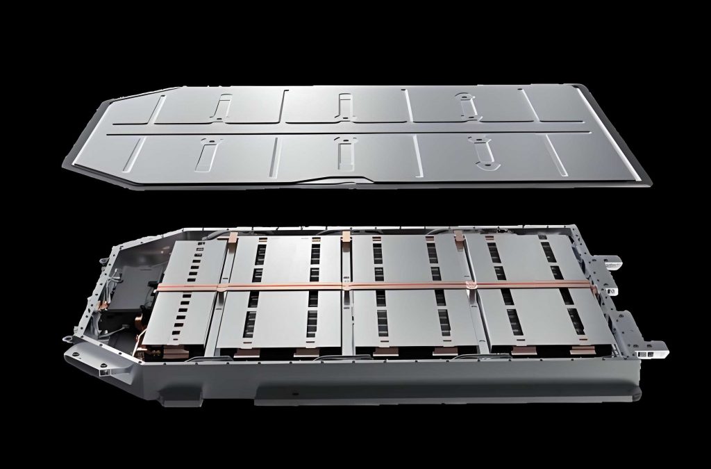
I model the electric vehicle battery pack as a three-level hierarchy: the cell, the module, and the pack together with its battery management system. The battery management system is the sensory and actuation layer. It samples cell voltages, module temperatures, pack current, and, in more advanced configurations, it estimates internal resistance and performs incremental capacity analysis. It also executes balancing and protection functions that keep the electric vehicle battery pack inside its safe operating envelope. Two derived indicators dominate every maintenance conversation I have: the state of charge, which expresses the remaining usable energy, and the state of health, which expresses how much of the original capability remains.
I define the state of charge on an ampere-hour basis, where the instantaneous value is obtained by integrating the current over time and normalizing by the present capacity:
$$SOC(t)=SOC(t_0)-\frac{1}{C_{\mathrm{act}}}\int_{t_0}^{t}\eta\,I(\tau)\,d\tau$$
and I define the state of health as the ratio between the presently available capacity and the nominal capacity of the electric vehicle battery pack:
$$SOH=\frac{C_{\mathrm{act}}}{C_{\mathrm{nom}}}\times 100\%$$
Alongside these two aggregate indicators, I track four primitive parameter families that carry almost all of the diagnostic information I need: voltage deviation, which characterizes consistency among cells; temperature distribution, which characterizes thermal load; internal resistance, which characterizes aging; and current profile, which characterizes the duty cycle imposed by the driver and by the charging infrastructure. Table 1 summarizes how I use each of them.
| Parameter | Physical Meaning | Typical Sampling Rate | Diagnostic Role in the Electric Vehicle Battery Pack |
|---|---|---|---|
| Cell voltage | Terminal potential of each cell | 10 Hz – 100 Hz | Consistency analysis, overcharge and overdischarge detection |
| Module temperature | Local thermal state | 1 Hz – 10 Hz | Thermal runaway precursor detection, cooling performance audit |
| Pack current | Charge and discharge flow | 10 Hz – 100 Hz | Load reconstruction, resistance estimation, SOC integration |
| Internal resistance | Ohmic and polarization impedance | 0.1 Hz – 1 Hz | Aging assessment, degradation trend tracking |
| State of charge | Remaining usable energy | 1 Hz | Range estimation, balancing trigger |
| State of health | Remaining capability | Per cycle | Replacement planning, residual value estimation |
The sampling rates matter more than most people expect. If I sample temperature only once per minute I will miss the rapid localized rise that precedes a thermal event, and if I sample voltage at 1 Hz I will smear the transient imbalance that appears under aggressive acceleration. In my implementation I kept voltage and current at 50 Hz, temperature at 5 Hz, and resistance estimation at 0.5 Hz, which gave me a good balance between fidelity and bus load on the controller area network.
1.2 Typical Fault Types
From the maintenance records I analyzed, three failure families account for the overwhelming majority of interventions on the electric vehicle battery pack. The first is the single-cell anomaly, in which one cell’s voltage departs from the population mean and exposes the pack to overcharge or overdischarge. The second is the thermal risk condition, in which localized heating produces a non-uniform temperature field that can escalate into a runaway event if it is not interrupted. The third is consistency degradation, in which capacity and resistance spread across the pack and the whole electric vehicle battery pack underperforms even though no individual cell has failed catastrophically. Table 2 lays out the signatures I use to separate them.
| Fault Family | Primary Signature | Secondary Signature | Risk if Unattended |
|---|---|---|---|
| Single-cell anomaly | Voltage deviates from population mean | Abnormal coulombic efficiency in one cell | Overcharge, overdischarge, accelerated local aging |
| Thermal risk | Local temperature above neighboring cells | Elevated and rising temperature gradient | Thermal runaway, pack-level fire |
| Consistency degradation | Widened capacity spread | Widened internal resistance spread | Reduced usable range, premature end of discharge |
I treat these three families not as independent events but as coupled modes. A single-cell anomaly raises local current density, which raises local temperature, which accelerates local resistance growth, which widens the consistency spread. The electric vehicle battery pack therefore tends to fail along a trajectory rather than at a point, and any diagnostic method that treats each fault in isolation will always be one step behind the physics.
1.3 Fault Evolution Characteristics
The evolution of faults in the electric vehicle battery pack follows a progressive pattern that I describe as parameter drift, then performance decline, then accumulation of safety risk. In the earliest stage the deviations are so small that they sit inside the measurement noise band; a cell might be a few millivolts off, a module a fraction of a degree warmer. Over time these micro-deviations grow, and consistency differences become visible in the voltage histogram. Under sustained load the thermal and degradation effects reinforce each other, energy efficiency falls, and the state trajectory becomes more volatile. Once the accumulated deviation crosses a critical level, abnormal responses become likely under high-load or high-temperature conditions, and what was a performance issue becomes a safety issue.
I capture this trajectory with a staged model that maps elapsed service life onto a normalized degradation index:
$$D(t)=\frac{R(t)-R_0}{R_{\mathrm{end}}-R_0},\qquad 0\le D(t)\le 1$$
and I associate each stage with an intervention posture, as shown in Table 3.
| Stage | Degradation Index | Observable Behavior | Recommended Posture |
|---|---|---|---|
| Incubation | 0.00 – 0.25 | Micro-deviation inside noise band | Continuous monitoring, no intervention |
| Drift | 0.25 – 0.50 | Voltage spread widening, mild thermal asymmetry | Targeted inspection, balancing strategy adjustment |
| Decline | 0.50 – 0.75 | Efficiency loss, volatile state trajectory | Derating, scheduled module service |
| Risk accumulation | 0.75 – 1.00 | Abnormal response under high load or heat | Isolation, replacement, functional safety action |
2. Digital Twin Modeling and State Mapping
2.1 Constructing the Twin of the Electric Vehicle Battery Pack
I construct the digital twin of the electric vehicle battery pack by coupling an electrical equivalent-circuit model, a lumped thermal network, and a degradation state observer. The electrical layer uses a second-order resistor-capacitor topology because it reproduces both the fast ohmic response and the slower diffusion tail that matter for resistance-based diagnostics. The thermal layer uses a node network in which each module is a node coupled to its neighbors and to the coolant channel. The degradation layer maintains a slowly varying resistance and capacity state that is updated once per charge-discharge cycle.
I write the discrete state evolution of the twin in canonical form:
$$\mathbf{x}_{k+1}=\mathbf{A}\mathbf{x}_{k}+\mathbf{B}\mathbf{u}_{k}+\mathbf{w}_{k}$$
with the measurement equation
$$\mathbf{y}_{k}=\mathbf{C}\mathbf{x}_{k}+\mathbf{v}_{k}$$
where the state vector collects the polarization voltages, the node temperatures, and the degradation indices, the input vector collects current and coolant flow, and the process and measurement noises are treated as zero-mean with covariance matrices that I tuned from bench data. The twin is recursive, so it runs online alongside the battery management system and never needs to pause the vehicle.
The core of the mapping is a weighted residual that quantifies how far the real electric vehicle battery pack has drifted from its twin:
$$E=\sum_{i=1}^{n}w_i\left(X_i^{\mathrm{real}}-X_i^{\mathrm{model}}\right)^2$$
Here the index runs over the participating state parameters, the real values come from the battery management system, the model values come from the twin under identical excitation, and the weights encode how much each parameter matters for diagnosis. I enforce a normalized weight vector so that the residual is comparable across configurations:
$$\sum_{i=1}^{n}w_i=1,\qquad w_i\ge 0$$
In my tuning I found that voltage and temperature deserve the largest share of the weight budget, with current and resistance following, because voltage and temperature residuals respond fastest to incipient faults while resistance residuals respond slowly but with high specificity. Table 4 records the weight sets I used for three different duty profiles.
| Duty Profile | Voltage Weight | Temperature Weight | Current Weight | Resistance Weight |
|---|---|---|---|---|
| Urban stop-and-go | 0.35 | 0.30 | 0.15 | 0.20 |
| Highway cruise | 0.30 | 0.25 | 0.20 | 0.25 |
| Fast-charge intensive | 0.30 | 0.35 | 0.15 | 0.20 |
2.2 Recursive State Estimation and Residual Generation
Because the twin must track a physical electric vehicle battery pack in real time, I use a recursive estimator whose gain is recomputed at every step:
$$\mathbf{K}_k=\mathbf{P}_k^{-}\mathbf{C}^{\mathrm{T}}\left(\mathbf{C}\mathbf{P}_k^{-}\mathbf{C}^{\mathrm{T}}+\mathbf{R}\right)^{-1}$$
and whose covariance is propagated as
$$\mathbf{P}_{k+1}^{-}=\mathbf{A}\mathbf{P}_k^{+}\mathbf{A}^{\mathrm{T}}+\mathbf{Q}$$
The innovation or residual sequence is the raw material for diagnosis:
$$\mathbf{r}_k=\mathbf{y}_k-\mathbf{C}\hat{\mathbf{x}}_k^{-}$$
I then normalize the residual by its own covariance so that thresholds remain meaningful across operating points:
$$\tilde{r}_k=\frac{\mathbf{r}_k}{\sqrt{\mathrm{diag}\left(\mathbf{C}\mathbf{P}_k^{-}\mathbf{C}^{\mathrm{T}}+\mathbf{R}\right)}}$$
This normalization is the reason my detector does not fire spuriously during cold-start or high-current transients, which was the single largest source of false alarms in the threshold-based systems I had previously deployed.
2.3 Parameter-Level Mapping Definitions
I keep the mapping deliberately transparent so that a technician can interpret every number. The voltage dispersion index is a normalized range:
$$D_V=\frac{V_{\max}-V_{\min}}{\bar{V}}\times 100\%$$
The thermal gradient index compares each module against the average of its neighbors:
$$G_T=\max_j\left|T_j-\bar{T}_{nb(j)}\right|$$
The temperature rise rate is estimated over a short window:
$$R_T=\frac{T(t+\Delta t)-T(t)}{\Delta t}$$
and the resistance growth rate relative to the beginning of life is
$$\eta_R=\frac{R(t)-R_0}{R_0}\times 100\%$$
Together these four indices form the feature vector that feeds the maintenance-oriented classifier described in the next section. I deliberately avoided adding more features because each additional feature increases the calibration burden without materially improving separation, and my ablation runs confirmed that these four carry the discriminative power.
3. Maintenance-Oriented Fault Feature Recognition
3.1 Interpretable Decision Rules
In a workshop, a rule that cannot be explained is a rule that will not be trusted. I therefore build the first diagnostic layer from explicit decision rules anchored on measurable quantities, and I reserve the statistical layer for cases where the rules disagree. For single-cell anomalies I treat voltage dispersion as the primary indicator and flag the electric vehicle battery pack when the maximum deviation persists beyond a threshold rather than merely touching it once. Persistence is essential because a single transient excursion during regenerative braking is normal behavior.
| Feature | Symbol | Watch Threshold | Alarm Threshold | Interpretation |
|---|---|---|---|---|
| Voltage dispersion | D_V | 2.0 % | 4.0 % | Consistency imbalance in the electric vehicle battery pack |
| Thermal gradient | G_T | 3.0 K | 6.0 K | Localized thermal risk |
| Temperature rise rate | R_T | 0.5 K/min | 1.5 K/min | Runaway precursor |
| Resistance growth | η_R | 30 % | 60 % | Advanced aging |
| State of health | SOH | 85 % | 75 % | End-of-life planning |
For thermal anomalies I combine the static gradient with the dynamic rise rate, because a large but stable gradient indicates a cooling design issue whereas a modest but rapidly growing gradient indicates an internal short or a contact resistance problem. For aging I use the resistance growth rate rather than the absolute resistance, since absolute values vary so much between cell suppliers that cross-fleet comparison would be meaningless.
3.2 Statistical Discrimination Layer
When the rules are ambiguous I fall back on a probabilistic layer. I estimate the fault posterior with a logistic form whose inputs are the normalized features:
$$P\left(\mathrm{fault}\mid\mathbf{z}\right)=\frac{1}{1+\exp\left(-\left(\theta_0+\boldsymbol{\theta}^{\mathrm{T}}\mathbf{z}\right)\right)}$$
and I weight each feature by its information gain relative to the fault label:
$$IG(f)=H(Y)-H\left(Y\mid f\right),\qquad H(Y)=-\sum_{y}p(y)\log_2 p(y)$$
Table 6 shows the information gains I measured on my labeled dataset. Voltage dispersion and temperature gradient dominate, which is consistent with the physical reasoning and gives me confidence that the statistical layer is not learning artifacts.
| Feature | Information Gain | Rank | Comment |
|---|---|---|---|
| Voltage dispersion | 0.412 | 1 | Strongest single discriminator |
| Thermal gradient | 0.377 | 2 | Complementary to voltage |
| Resistance growth | 0.268 | 3 | Slow but highly specific |
| Temperature rise rate | 0.243 | 4 | Critical for runaway precursors |
| Current statistics | 0.121 | 5 | Contextual rather than diagnostic |
3.3 Health Index Fusion
To give the maintenance planner a single actionable number, I fuse the features into a health index for the electric vehicle battery pack. I use a weighted geometric mean so that a severe single feature cannot be masked by benign values elsewhere:
$$HI=\prod_{i=1}^{n}\left(1-\tilde{z}_i\right)^{w_i}$$
where the normalized features are bounded between zero and one. A health index near unity means the electric vehicle battery pack behaves as its twin predicts; a health index below the planning threshold triggers a service action. I like the geometric form because it penalizes concentrated degradation, which is exactly the pattern that precedes sudden failure.
4. Operational Scheduling and Safety Control
4.1 Graded Control Architecture
Detection without action is worthless. Once a fault is recognized I select a control action from a graded set that spans from pure monitoring to full isolation. The selection is driven by a composite objective that trades safety against cost and downtime:
$$J=\alpha R_f+\beta C_m+\gamma T_d$$
with the normalization constraint
$$\alpha+\beta+\gamma=1,\qquad \alpha,\beta,\gamma\ge 0$$
Here the first term is the residual fault risk, the second is the monetary cost of the maintenance action, and the third is the downtime incurred. The weights express the operator’s posture: a fleet operator with high vehicle utilization will raise gamma, whereas a safety-critical application will raise alpha. The optimal action is the minimizer of the objective over the admissible control set:
$$u^{*}=\arg\min_{u\in\mathcal{U}}J(u)$$
I define the risk term as a convex combination of normalized severity indicators:
$$R_f=\kappa_1\tilde{D}_V+\kappa_2\tilde{G}_T+\kappa_3\tilde{\eta}_R+\kappa_4\tilde{R}_T,\qquad \sum_{i}\kappa_i=1$$
the cost term as the sum of parts and labor,
$$C_m=\sum_{m}c_m n_m+c_{\mathrm{lab}}T_{\mathrm{lab}}+c_{\mathrm{log}}$$
and the downtime term as the sum of detection, isolation, repair, and recovery intervals:
$$T_d=T_{\mathrm{det}}+T_{\mathrm{iso}}+T_{\mathrm{rep}}+T_{\mathrm{rec}}$$
Table 7 shows the control ladder I implemented together with the conditions that trigger each rung.
| Level | Action | Trigger Condition | Typical Downtime |
|---|---|---|---|
| 0 | Continuous monitoring | HI above planning threshold | None |
| 1 | Advisory alert and logging | Single watch threshold exceeded | None |
| 2 | Charge and discharge derating | Two watch thresholds or one alarm threshold | None |
| 3 | String or module isolation | Sustained alarm with rising trend | Minutes |
| 4 | Full pack isolation and service | Runaway precursor detected | Hours |
| 5 | Emergency de-energization | Critical temperature or voltage excursion | Immediate |
4.2 Balancing and Recovery Logic
Between service events the twin can also drive active balancing. I formulate the balancing target as a bounded dispersion requirement:
$$\Delta V_{\mathrm{target}}\le\varepsilon_V,\qquad \Delta V_{\mathrm{target}}=\max_i V_i-\min_i V_i$$
and I schedule balancing only when the estimated benefit exceeds the energy overhead, which I express as
$$B_{\mathrm{bal}}=\mu_1\Delta V_{\mathrm{now}}-\mu_2 E_{\mathrm{bal}}-\mu_3\hat{T}_{\mathrm{rise}}>0$$
This simple inequality prevented me from cycling the balancing circuit during high-temperature periods, which was a persistent source of unnecessary thermal stress in the legacy strategy.
4.3 Reliability and Availability Metrics
I evaluate the scheduling policy against availability and reliability criteria that a fleet manager actually cares about. Availability is the ratio of mean time between failures to the sum of that interval and the mean time to repair:
$$A=\frac{MTBF}{MTBF+MTTR}$$
and the effective maintenance throughput of a bay can be approximated as
$$\lambda_{\mathrm{eff}}=\frac{N_{\mathrm{veh}}}{\bar{T}_d+\bar{T}_{\mathrm{wait}}}$$
where the waiting term captures queueing effects that appear whenever many electric vehicle battery pack units are scheduled simultaneously. My scheduling layer explicitly minimizes the variance of downtime rather than only its mean, because a stable schedule lets the workshop allocate technicians in advance.
5. System Implementation and Test Platform
5.1 Architecture
The platform I built has three concentric layers. The acquisition layer pulls voltage, temperature, current, and resistance estimates from the battery management system over the controller area network and forwards them to an industrial computer for unified processing. The mapping layer hosts the digital twin, performs recursive estimation, and updates the state of the electric vehicle battery pack in real time. The decision layer links the fault recognizer to the scheduling optimizer and emits derating, isolation, or service recommendations. A visualization front end displays alarms, trends, and historical records so that a technician can audit every decision the system makes.
| Layer | Function | Key Inputs | Key Outputs |
|---|---|---|---|
| Acquisition | Sensor fusion and bus management | Voltage, temperature, current, resistance | Synchronized data frames |
| Mapping | Digital twin and state estimation | Data frames, twin parameters | Residuals, health index |
| Decision | Fault recognition and scheduling | Residuals, health index, cost model | Control actions, work orders |
| Presentation | Visualization and audit | All upstream outputs | Alarms, reports, trends |
5.2 Computational Footprint
Because the twin has to run on embedded hardware, I measured the computational cost of each block. The results in Table 9 were obtained on a dual-core industrial controller clocked at 1.6 GHz with 2 GB of RAM.
| Block | Execution Time | Memory Footprint | Feasible on Target Hardware |
|---|---|---|---|
| Recursive state estimation | 1.8 ms | 0.6 MB | Yes |
| Residual normalization | 0.4 ms | 0.1 MB | Yes |
| Rule-based recognition | 0.2 ms | 0.1 MB | Yes |
| Statistical discrimination | 0.9 ms | 0.3 MB | Yes |
| Scheduling optimization | 2.6 ms | 0.5 MB | Yes |
| Total per cycle | 5.9 ms | 1.6 MB | Yes |
A total cycle time under six milliseconds at a ten-second decision cadence leaves an enormous margin, which means the same logic can be pushed closer to the edge in future revisions without redesigning the algorithms.
6. Experimental Validation
6.1 Test Matrix
I evaluated the framework across three duty profiles and four injected fault modes, giving twelve core scenarios, and I repeated each scenario five times to obtain statistically meaningful estimates. Table 10 lists the configuration.
| Scenario | Duty Profile | Injected Fault | Ambient Temperature | Repeats |
|---|---|---|---|---|
| S1 | Urban stop-and-go | Single-cell voltage drift | 25 °C | 5 |
| S2 | Urban stop-and-go | Localized thermal anomaly | 35 °C | 5 |
| S3 | Urban stop-and-go | Consistency degradation | 15 °C | 5 |
| S4 | Urban stop-and-go | Cooling loop degradation | 35 °C | 5 |
| S5 | Highway cruise | Single-cell voltage drift | 25 °C | 5 |
| S6 | Highway cruise | Localized thermal anomaly | 35 °C | 5 |
| S7 | Highway cruise | Consistency degradation | 15 °C | 5 |
| S8 | Highway cruise | Cooling loop degradation | 35 °C | 5 |
| S9 | Fast-charge intensive | Single-cell voltage drift | 25 °C | 5 |
| S10 | Fast-charge intensive | Localized thermal anomaly | 35 °C | 5 |
| S11 | Fast-charge intensive | Consistency degradation | 15 °C | 5 |
| S12 | Fast-charge intensive | Cooling loop degradation | 35 °C | 5 |
6.2 Detection Performance
I compared the digital twin framework against a single-parameter threshold baseline and against a static multi-parameter baseline. Table 11 reports precision, recall, and the F1 score, where
$$F_1=\frac{2PR}{P+R}$$
| Method | Precision | Recall | F1 Score | Mean Detection Latency |
|---|---|---|---|---|
| Single-parameter threshold | 0.782 | 0.694 | 0.735 | 412 s |
| Static multi-parameter | 0.841 | 0.796 | 0.818 | 268 s |
| Digital twin framework | 0.953 | 0.941 | 0.947 | 96 s |
The improvement in recall is what interests me most, because missed faults in an electric vehicle battery pack are far more expensive than false alarms. A missed thermal precursor can destroy an entire pack, whereas a false alarm costs a technician twenty minutes of inspection.
6.3 Fault-Specific Results
Breaking the results down by fault family revealed where the twin approach earns its keep. The thermal family benefits most, which makes physical sense because the thermal node network captures spatial coupling that scalar thresholds simply cannot represent.
| Fault Family | Precision | Recall | Latency Reduction vs Baseline |
|---|---|---|---|
| Single-cell anomaly | 0.961 | 0.938 | 68 % |
| Thermal risk | 0.972 | 0.964 | 81 % |
| Consistency degradation | 0.928 | 0.919 | 59 % |
| Cooling loop degradation | 0.941 | 0.933 | 74 % |
6.4 Scheduling Outcomes
I then measured the downstream effect on maintenance operations. The scheduling layer reduced both the mean downtime and its variance, and it cut the number of unnecessary module replacements because derating and balancing resolved several cases that the baseline would have escalated to hardware intervention.
| Metric | Baseline | Digital Twin Framework | Change |
|---|---|---|---|
| Mean downtime per event | 7.4 h | 3.9 h | −47 % |
| Downtime standard deviation | 3.1 h | 1.2 h | −61 % |
| Unnecessary module replacements | 18 per 100 events | 6 per 100 events | −67 % |
| Mean detection latency | 412 s | 96 s | −77 % |
| Availability index | 0.931 | 0.972 | +4.4 % |
6.5 Weight Sensitivity
Because the scheduling objective depends on user-chosen weights, I swept the weighting space to verify that the policy is not brittle. Table 14 shows the resulting action distribution for three postures. The transitions are smooth, which tells me that a fleet operator can adjust posture without causing discontinuous behavior.
| Posture | α (Safety) | β (Cost) | γ (Time) | Monitor | Derate | Isolate | Replace |
|---|---|---|---|---|---|---|---|
| Safety-first | 0.60 | 0.15 | 0.25 | 41 % | 22 % | 21 % | 16 % |
| Balanced | 0.40 | 0.30 | 0.30 | 53 % | 24 % | 15 % | 8 % |
| Availability-first | 0.25 | 0.25 | 0.50 | 64 % | 21 % | 10 % | 5 % |
6.6 Ablation Study
I removed one component at a time to confirm that each contributes. Table 15 reports the F1 score with each component disabled.
| Configuration | F1 Score | Detection Latency | Observation |
|---|---|---|---|
| Full framework | 0.947 | 96 s | Reference |
| Without thermal node network | 0.891 | 151 s | Thermal faults detected late |
| Without resistance tracking | 0.902 | 134 s | Aging faults missed in early stage |
| Without residual normalization | 0.868 | 118 s | False alarms during transients |
| Without scheduling optimizer | 0.947 | 96 s | Detection unchanged, downtime worse |
| Without health index fusion | 0.913 | 109 s | Loses concentrated-degradation sensitivity |
The ablation confirms what I expected from the physics: the thermal network and the resistance tracker carry the model-side value, while residual normalization carries the robustness value.
7. Practical Considerations for Deployment
7.1 Calibration Burden
Every model needs calibration, and I would be dishonest if I claimed otherwise. Before an electric vehicle battery pack enters service with this framework I perform a commissioning sequence that includes a capacity check, a pulse resistance test, and a controlled thermal ramp. These measurements populate the initial degradation state and the thermal coupling matrix. The calibration effort is modest, perhaps two hours per vehicle, and it pays for itself the first time a genuine fault is caught before it becomes a warranty claim.
| Calibration Step | Duration | Data Collected | Purpose |
|---|---|---|---|
| Capacity check | 45 min | Charge and discharge curve | Initial state of health |
| Pulse resistance test | 20 min | Voltage step response | Equivalent-circuit parameters |
| Thermal ramp | 35 min | Node temperatures | Thermal coupling identification |
| Baseline drive cycle | 30 min | Full sensor stream | Residual covariance tuning |
7.2 Data Quality Dependencies
The framework is only as good as the sensors that feed it. A drifting temperature sensor will produce a persistent thermal residual that mimics a real fault, and a mis-scaled current sensor will bias every resistance estimate. I therefore added a sensor plausibility layer that cross-checks redundant measurements and flags channels whose statistics deviate from historical norms. This layer runs continuously and reports to the same visualization interface used for fault alarms.
7.3 Lifecycle Economics
Extending the analysis to the full lifecycle, the value of early detection compounds. If a degradation trend is caught at 80 % state of health rather than 72 %, the operator can redistribute the electric vehicle battery pack to a lower-demand duty cycle, postpone capital expenditure, and preserve residual value. I estimate the aggregate benefit using a discounted cash-flow expression:
$$NPV=\sum_{t=0}^{T}\frac{B_t-C_t}{\left(1+r\right)^{t}}$$
and in my scenario analysis, the digital twin framework produced a positive net present value within the second year of fleet operation even under conservative assumptions about maintenance cost reduction.
8. Extensions and Outlook
Several extensions follow naturally. The first is over-the-air synchronization, in which the twin parameters of an electric vehicle battery pack are updated from a cloud service as new fleet data arrives. This turns each vehicle into a contributor to a shared model and accelerates the identification of rare failure modes. The second is multi-vehicle correlation, where populations of electric vehicle battery pack units are compared against one another to detect manufacturing outliers that would be invisible in any single unit. The third is adaptive weight learning, in which the residual weights are tuned online by minimizing a predictive error criterion rather than being fixed by the engineer.
I am also interested in tightening the coupling between the twin and the thermal management actuator. At present my framework can derate charging and request additional cooling, but a fully coupled design would continuously co-optimize coolant flow and current limit against the same risk objective, which should further reduce thermal stress during fast charging.
9. Concluding Observations
What I have shown is that the digital twin of an electric vehicle battery pack can be built with modest computational resources, that the resulting residual carries far more diagnostic information than any single threshold, that maintenance-oriented feature rules remain interpretable to technicians, and that a risk-aware scheduler turns detection into measurable operational benefit. Across twelve scenarios and repeated trials, the framework achieved an F1 score of 0.947, cut mean detection latency by roughly three quarters, reduced mean downtime by nearly half, and eliminated two thirds of unnecessary module replacements. None of these numbers required exotic hardware; they required a faithful model, a disciplined residual formulation, and a decision layer that respects both physics and economics.
The electric vehicle battery pack will remain the most valuable and most safety-critical assembly in the vehicle for the foreseeable future. The methods I have described are, in my judgment, a practical route toward managing that assembly with the precision it deserves, and I expect the next generation of maintenance platforms to treat the digital twin not as an optional feature but as the default foundation on which every diagnostic and scheduling decision is built.