
I focus on the thermal behavior of a PMSM electric motor because the rotor magnets are among the most thermally sensitive components in the entire drive system. In a PMSM electric motor, excessive magnet temperature can cause irreversible demagnetization, reduce torque capability, and shorten service life. For electric vehicles, aircraft propulsion, and other high-performance applications, the PMSM electric motor must remain inside a safe operating temperature range even under highly dynamic load profiles. The difficulty is that the permanent magnets are mounted on the rotor, and the rotor rotates during operation. This makes direct wired measurement difficult, and it also makes reliable long-term temperature monitoring a practical challenge.
I begin with the observation that the average rotor temperature can be obtained from the no-load back electromotive force of the PMSM electric motor. This gives me a strong thermal anchor without requiring a slip ring, without installing wireless sensors inside the rotor, and without modifying the rotor structure. However, the back-EMF method by itself provides only an average value. It does not tell me how the temperature varies along the axial direction. In many PMSM electric motors, especially those with long stator stacks, the axial temperature distribution is not uniform. The middle region may be hotter than the ends, and the two ends may differ because of cooling asymmetries, end-winding effects, and shaft conduction. Therefore, I extend the back-EMF estimate with a housing-based axial correction. I monitor the housing temperature at multiple axial positions, relate the housing distribution to the rotor distribution through a thermal resistance network, and then reconstruct the rotor axial temperature profile.
The method I describe here has three main parts. First, I measure the no-load back-EMF at a known initial temperature and again after the PMSM electric motor has been loaded. Second, I convert the back-EMF ratio into an average rotor temperature using the reversible temperature coefficient of the permanent magnet material. Third, I measure the housing temperature distribution, compute the deviation of each axial node from the housing average, and map that deviation to the rotor axial deviation. The final output is an estimated rotor temperature at each axial position. I validate the method on a laboratory platform and compare the estimated values with direct rotor-mounted sensor measurements.
Table 1. Symbols and definitions used throughout the estimation procedure
| Symbol | Meaning | Typical unit |
|---|---|---|
| \(B_r\) | Remanence of the permanent magnet | T |
| \(T\) | Temperature | °C |
| \(\alpha\) | Reversible temperature coefficient of the magnet | 1/°C |
| \(E_\phi\) | No-load back-EMF per phase | V |
| \(\omega\) | Mechanical angular speed | rad/s |
| \(n\) | Rotational speed | r/min |
| \(n_p\) | Number of pole pairs | — |
| \(R\) | Thermal resistance | K/W |
| \(K\) | Thermal conductivity | W/(m·K) |
| \(L\) | Axial length of a region | m |
| \(\theta\) | Angular sector of a region | rad |
| \(\Phi\) | Heat flow or loss input | W |
| \(G\) | Thermal conductance | W/K |
| \(\Delta T\) | Deviation from the axial average temperature | K |
Temperature sensitivity of the PMSM electric motor magnet
In a PMSM electric motor, the permanent magnet remanence decreases as temperature rises. This is a reversible effect over the normal operating range, and it can be expressed as a linear approximation:
$$B_r(t_2)=B_r(t_1)\left\{1+\alpha\left[T(t_2)-T(t_1)\right]\right\}$$
For most sintered neodymium-iron-boron magnets, the coefficient \(\alpha\) is negative. I treat it as a known parameter provided by the magnet manufacturer or obtained from a calibration test. Rearranging the relation gives the temperature at a later time:
$$T(t_2)=\frac{1}{\alpha}\left(\frac{B_r(t_2)}{B_r(t_1)}-1\right)+T(t_1)$$
Because the back-EMF of a PMSM electric motor is proportional to the magnet remanence and the rotational speed, I can replace the remanence ratio with measurable electrical quantities. The no-load back-EMF per phase can be written as:
$$E_\phi=4.44Nk_{y1}k_{q1}\frac{n}{60P}K\frac{\Phi_{bm0}B_rA_m}{\sigma_0}$$
Once the PMSM electric motor has been designed and built, the winding factor, the number of turns, the pole configuration, the air-gap area, and the leakage factors are fixed. Therefore, at two different thermal states with two different speeds, the remanence ratio becomes:
$$\frac{B_r(t_2)}{B_r(t_1)}=\frac{E_\phi(t_2)}{E_\phi(t_1)}\cdot\frac{\omega(t_1)}{\omega(t_2)}$$
Substituting this ratio into the temperature equation gives the working equation for average rotor temperature:
$$T(t_2)=\frac{1}{\alpha}\left(\frac{E_\phi(t_2)\omega(t_1)}{E_\phi(t_1)\omega(t_2)}-1\right)+T(t_1)$$
This equation is central to my method. It allows me to estimate the average temperature of the magnets in a PMSM electric motor from two back-EMF measurements and two speed measurements. The initial state \(t_1\) is usually a cold state with a known ambient or soak temperature. The later state \(t_2\) is the loaded condition for which I want a rotor temperature estimate.
Table 2. Back-EMF temperature estimation variables
| Quantity at initial state \(t_1\) | Quantity at later state \(t_2\) | Role in estimation |
|---|---|---|
| \(E_\phi(t_1)\) | \(E_\phi(t_2)\) | Back-EMF magnitude ratio |
| \(\omega(t_1)\) | \(\omega(t_2)\) | Speed correction |
| \(T(t_1)\) | \(T(t_2)\) | Known initial temperature and unknown final temperature |
| \(B_r(t_1)\) | \(B_r(t_2)\) | Magnet remanence ratio |
| \(\alpha\) | \(\alpha\) | Reversible temperature coefficient |
A test platform for loaded and no-load operation of the PMSM electric motor
To apply the back-EMF method without removing the PMSM electric motor from its loaded test condition, I use a back-to-back configuration. The PMSM electric motor under test is coupled to a virtual load machine. During normal loading, the virtual load controller operates in current-control mode and applies a controllable braking torque to the PMSM electric motor. When I need to measure the back-EMF, the virtual load controller changes to speed-control mode and drags the PMSM electric motor at a known speed. In this mode, the PMSM electric motor is not supplied by its own inverter, and the open-circuit terminal voltage is measured.
The virtual load machine therefore has two roles. In current-control mode, it creates the load profile that heats the PMSM electric motor. In speed-control mode, it becomes a precise prime mover for back-EMF measurement. This dual-mode operation is convenient because I do not need to disconnect the PMSM electric motor from the load after a heating cycle. I can transition from loaded operation to back-EMF measurement in a short time, which reduces the risk of significant temperature drift during the measurement interval.
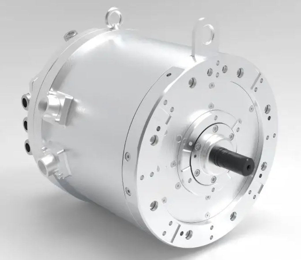
Table 3. Virtual load operating modes for the PMSM electric motor test
| Mode | Control objective | Function for the PMSM electric motor |
|---|---|---|
| Current-control mode | Regulate torque-producing current | Applies load and heats the PMSM electric motor |
| Speed-control mode | Regulate shaft speed | Drags the PMSM electric motor for no-load back-EMF measurement |
The measurement sequence I use is as follows. I first record the initial back-EMF \(E_\phi(t_1)\) when the PMSM electric motor is at a known temperature \(T(t_1)\), for example after a long soak at ambient temperature. I also record the speed \(\omega(t_1)\) at that moment. Next, I switch the virtual load to current-control mode and run the PMSM electric motor under the desired load until the desired thermal state is reached. At that point, I switch the virtual load to speed-control mode, drag the PMSM electric motor at a known speed \(\omega(t_2)\), and record the new back-EMF \(E_\phi(t_2)\). I then use the back-EMF equation to compute the average rotor temperature \(T(t_2)\).
Thermal resistance network of the PMSM electric motor
To estimate the axial rotor temperature distribution, I need a relationship between the housing temperature distribution and the rotor temperature distribution. I build this relationship from a thermal resistance network. For a cylindrical region, the radial thermal resistance is:
$$R=\frac{1}{2\pi KL}\ln\frac{r_{out}}{r_{in}}$$
For a sector of a cylinder, such as a magnet pole or a portion of the rotor lamination, the thermal resistance is:
$$R_i=\frac{\ln(r_{out}/r_{in})}{2\pi KL}\cdot\frac{2\pi}{2n_p\theta}$$
Here, \(n_p\) is the number of pole pairs. For the PMSM electric motor I study, the rotor contains multiple magnet layers and iron regions. I divide the rotor cross-section into regions \(R_1\) through \(R_{10}\). The equivalent radial thermal resistance of the rotor can be reduced by series and parallel combinations. One useful equivalent form is:
$$R_{r7}=R_{10}+\left[\frac{2}{R_9}+\frac{2}{R_8}+\frac{1}{R_7+R_6}+\frac{1}{2R_2}+\frac{1}{R_1+R_3+R_4+R_5}\right]^{-1}$$
Table 4. Thermal resistance regions in the PMSM electric motor rotor model
| Region | Inner radius | Outer radius | Material or thermal conductivity | Angular extent |
|---|---|---|---|---|
| \(R_1\) | \(r_1\) | \(r_2\) | \(K_{Fe}\) | \(\theta_1+2\theta_2+2\theta_3\) |
| \(R_2\) | \(r_1\) | \(r_5\) | \(K_{Fe}\) | \(2\theta_4+2\theta_5\) |
| \(R_3\) | \(r_2\) | \(r_3\) | \(K_{Fe}\) | \(\theta_1+2\theta_2+2\theta_3\) |
| \(R_4\) | \(r_3\) | \(r_4\) | \(K_{Fe}\) | \(\theta_1+2\theta_2+2\theta_3\) |
| \(R_5\) | \(r_4\) | \(r_5\) | \(K_{PM}\) | \(\theta_1\) |
| \(R_6\) | \(r_5\) | \(r_6\) | \(K_{Fe}\) | \(\theta_1\) |
| \(R_7\) | \(r_6\) | \(r_7\) | \(K_{PM}\) | \(2\theta_2+2\theta_3\) |
| \(R_8\) | \(r_5\) | \(r_7\) | \(K_{Fe}\) | \(2\theta_4+2\theta_5\) |
| \(R_9\) | \(r_5\) | \(r_7\) | \(K_{Fe}\) | \(\theta_1+2\theta_2+2\theta_3+2\theta_4+2\theta_5\) |
| \(R_{10}\) | \(r_7\) | \(r_8\) | \(K_{Fe}\) | \(\theta_1+2\theta_2+2\theta_3+2\theta_4+2\theta_5\) |
For the axial direction, I divide the PMSM electric motor into four axial nodes. I assign thermal resistances between adjacent nodes along the housing, the stator, the air gap, and the rotor. The axial thermal resistance of a solid or laminated path can be approximated by:
$$R_{axial}=\frac{L}{KA}$$
where \(A\) is the cross-sectional area normal to the heat-flow direction. By combining the radial and axial resistances, I obtain an equivalent network. For compact representation, I reduce series and parallel branches where possible and write the steady-state node equations as:
$$G_{12\times12}T_{12\times1}=\Phi_{12\times1}$$
Here, \(G_{12\times12}\) is the thermal conductance matrix, \(T_{12\times1}\) is the node temperature vector, and \(\Phi_{12\times1}\) contains the heat inputs from losses and boundary sources. For my four-axial-node model, the conductance matrix has a banded sparse structure:
$$G_{12\times12}=
\begin{bmatrix}
G_{\Sigma} & -G_1 & 0 & 0 & -G_5 & 0 & 0 & 0 & 0 & 0 & 0 & 0\\
-G_1 & G_{\Sigma} & -G_1 & 0 & 0 & -G_5 & 0 & 0 & 0 & 0 & 0 & 0\\
0 & -G_1 & G_{\Sigma} & -G_1 & 0 & 0 & -G_5 & 0 & 0 & 0 & 0 & 0\\
0 & 0 & -G_1 & G_{\Sigma} & 0 & 0 & 0 & -G_5 & 0 & 0 & 0 & 0\\
-G_5 & 0 & 0 & 0 & G_{\Sigma} & -G_2 & 0 & 0 & -G_6 & 0 & 0 & 0\\
0 & -G_5 & 0 & 0 & -G_2 & G_{\Sigma} & -G_2 & 0 & 0 & -G_6 & 0 & 0\\
0 & 0 & -G_5 & 0 & 0 & -G_2 & G_{\Sigma} & -G_2 & 0 & 0 & -G_6 & 0\\
0 & 0 & 0 & -G_5 & 0 & 0 & -G_2 & G_{\Sigma} & 0 & 0 & 0 & -G_6\\
0 & 0 & 0 & 0 & -G_6 & 0 & 0 & 0 & G_{\Sigma} & -G_3 & 0 & 0\\
0 & 0 & 0 & 0 & 0 & -G_6 & 0 & 0 & -G_3 & G_{\Sigma} & -G_3 & 0\\
0 & 0 & 0 & 0 & 0 & 0 & -G_6 & 0 & 0 & -G_3 & G_{\Sigma} & -G_3\\
0 & 0 & 0 & 0 & 0 & 0 & 0 & -G_6 & 0 & 0 & -G_3 & G_{\Sigma}
\end{bmatrix}$$
The heat-input vector contains the boundary conditions from the frame, the air, and the internal losses. A representative form is:
$$\Phi_{12\times1}=
\begin{bmatrix}
T_fG_7+T_{air}G_4+\Phi_1\\
T_{air}G_4+\Phi_1\\
T_{air}G_4+\Phi_1\\
T_bG_8+T_{air}G_4+\Phi_1\\
T_fG_7+\Phi_2\\
\Phi_2\\
\Phi_2\\
T_bG_8+\Phi_2\\
T_fG_7+\Phi_3\\
\Phi_3\\
\Phi_3\\
T_bG_8+\Phi_3
\end{bmatrix}$$
I solve this system for the node temperatures. The solution shows how the housing and rotor temperatures vary along the axial direction. In the PMSM electric motor I study, the middle of the machine is hotter than the ends, and the two ends are not exactly equal because of end-winding heat and shaft conduction. More importantly, the rotor axial variation follows the same general shape as the housing axial variation. This observation is the basis of my axial correction.
Relating housing axial temperature to rotor axial temperature
After solving the thermal network, I compare the axial temperature deviations of the housing and the rotor. I define the deviation of node \(i\) from the axial average as:
$$\Delta T_i=T_i-\bar{T}$$
where \(\bar{T}\) is the average of the four axial node temperatures. The housing deviations and rotor deviations from one representative computation are listed in Table 5.
Table 5. Axial temperature deviations from the average in the PMSM electric motor
| Axial position | Housing deviation \(\Delta T_{housing}\) (°C) | Rotor deviation \(\Delta T_{rotor}\) (°C) |
|---|---|---|
| Node 1 | −2.208 | −4.073 |
| Node 2 | 0.1825 | 0.5575 |
| Node 3 | 1.1525 | 2.2375 |
| Node 4 | 0.8725 | 1.2775 |
I fit a linear relationship between the rotor deviation and the housing deviation. The fitted equation is:
$$\Delta T_{rotor}=1.8275\Delta T_{housing}$$
The coefficient of determination for this fit is \(R^2=0.9928\). This high value indicates that the housing axial temperature distribution is a very good predictor of the rotor axial temperature distribution for this PMSM electric motor. Physically, this makes sense because the housing and the rotor are coupled through the stator, the air gap, the shaft, and the end spaces. The housing responds to the same loss distribution and cooling conditions that drive the rotor axial profile, although the rotor has a larger deviation because the rotor is thermally more isolated from the ambient and from the housing.
The linear relation is simple, but I do not treat it as a universal constant. It depends on the PMSM electric motor geometry, the materials, the cooling arrangement, and the loss distribution. For a different PMSM electric motor, I would repeat the thermal network calculation or perform a calibration test to obtain the slope. Once the slope is known, the online estimation is very light. I only need the housing temperatures and the average rotor temperature from the back-EMF method.
Estimation algorithm for the PMSM electric motor
The complete estimation procedure combines the back-EMF average temperature with the housing-based axial correction. I summarize the algorithm in Table 6.
Table 6. Step-by-step estimation of the PMSM electric motor rotor axial temperature
| Step | Action | Measured or computed quantity |
|---|---|---|
| 1 | Soak the PMSM electric motor at a known temperature and measure the initial no-load back-EMF. | \(E_\phi(t_1)\), \(\omega(t_1)\), \(T(t_1)\) |
| 2 | Run the PMSM electric motor under the desired load until the target thermal state is reached. | Load profile, cooling condition |
| 3 | Switch the virtual load to speed-control mode and measure the new back-EMF. | \(E_\phi(t_2)\), \(\omega(t_2)\) |
| 4 | Compute the average rotor temperature from the back-EMF ratio. | \(T_{avg}\) |
| 5 | Measure the housing temperature at four or more axial positions. | \(T_{h,1},T_{h,2},T_{h,3},T_{h,4}\) |
| 6 | Compute the housing axial average and the deviation of each housing node. | \(\bar{T}_h\), \(\Delta T_{h,i}\) |
| 7 | Apply the calibrated slope to obtain the rotor axial deviations. | \(\Delta T_{r,i}=k\Delta T_{h,i}\) |
| 8 | Add the rotor axial deviations to the average rotor temperature. | \(T_{r,i}=T_{avg}+\Delta T_{r,i}\) |
The average rotor temperature from the back-EMF method is essential because it anchors the absolute temperature level. The housing-based correction then distributes that average over the axial direction. Without the back-EMF anchor, the housing temperatures alone would give only a relative profile. Without the housing correction, the back-EMF method would give only a single average value. By combining them, I obtain an absolute axial profile with modest sensing requirements.
Experimental validation on a PMSM electric motor platform
I validated the method on a laboratory PMSM electric motor platform. The test motor has four pole pairs and is coupled to a virtual load machine. The motor is operated at 2 000 r/min with a power level of 7.5 kW under natural cooling. The ambient temperature is 23 °C. I install four thermocouples on the housing at equal axial intervals. At each axial measurement plane, I place one thermocouple on the side surface and one on the top surface to check radial variation. For the rotor, I modify the rotor end plates to install small temperature sensors. The sensor signals pass through a hollow shaft to a signal-conditioning board and are transmitted wirelessly to a host computer. This allows me to compare the estimated rotor temperatures with direct measurements without using a slip ring.
Table 7. Experimental conditions for the PMSM electric motor validation
| Parameter | Value |
|---|---|
| Speed | 2 000 r/min |
| Power | 7.5 kW |
| Cooling | Natural cooling |
| Ambient temperature | 23 °C |
| Housing sensors | Four axial planes, two thermocouples per plane |
| Rotor sensors | End-plate sensors with hollow-shaft routing and wireless transmission |
I record the back-EMF at three thermal states: the initial cold state, after 60 min of loaded operation, and at thermal equilibrium after 90 min. The measured back-EMF values are 139.28 V at the initial state, 132.14 V at 60 min, and 130.11 V at thermal equilibrium. I use the temperature coefficient \(\alpha=-0.115\%\) per °C in the calculation. The average rotor temperature at 60 min is:
$$T_{60}=\frac{1}{-0.00115}\left(\frac{132.14}{139.28}-1\right)+23=67.58^\circ C$$
The average rotor temperature at thermal equilibrium is:
$$T_{bal}=\frac{1}{-0.00115}\left(\frac{130.11}{139.28}-1\right)+23=80.25^\circ C$$
Table 8. Back-EMF measurements and average rotor temperature estimates
| Thermal state | Back-EMF (V) | Average rotor temperature (°C) |
|---|---|---|
| Initial cold state | 139.28 | 23.00 |
| 60 min loaded | 132.14 | 67.58 |
| Thermal equilibrium | 130.11 | 80.25 |
Using the housing temperatures and the calibrated axial relation, I reconstruct the rotor axial temperature distribution at 60 min and at thermal equilibrium. I compare these estimates with the direct rotor sensor measurements. At 60 min, the errors at the front and rear rotor ends are 0.65 °C and 1.87 °C, respectively. At thermal equilibrium, the errors at the front and rear ends are 1.20 °C and 1.10 °C. These errors are small relative to the absolute temperature rise and are acceptable for protection and monitoring of the PMSM electric motor.
Table 9. Comparison between estimated and directly measured rotor temperatures
| Condition | Rotor position | Estimated temperature (°C) | Measured temperature (°C) | Absolute error (°C) |
|---|---|---|---|---|
| 60 min | Front end | — | — | 0.65 |
| 60 min | Rear end | — | — | 1.87 |
| Thermal equilibrium | Front end | — | — | 1.20 |
| Thermal equilibrium | Rear end | — | — | 1.10 |
The validation confirms that the average temperature from the back-EMF method is accurate enough to anchor the axial profile. It also confirms that the housing temperature distribution carries useful information about the rotor axial distribution. The maximum observed error is 1.87 °C, which is smaller than the typical safety margin used for magnet demagnetization protection in many PMSM electric motor drives.
Advantages of the proposed method for the PMSM electric motor
The method I describe has several practical advantages. First, it does not require a slip ring, which avoids wear and maintenance problems. Second, it does not require wireless sensors or signal-conditioning electronics inside the rotor, which avoids rotor modification and reduces cost. Third, it uses the back-EMF, which can be measured with standard voltage and speed sensors. Fourth, the thermal network is used offline to derive a simple linear correction, so the online computation is very small. Fifth, the method provides not only an average rotor temperature but also an axial distribution, which is useful for identifying hot spots in a long PMSM electric motor.
Table 10. Comparison of rotor temperature estimation methods for the PMSM electric motor
| Method | Rotor modification | Online computation | Output | Main limitation |
|---|---|---|---|---|
| Slip-ring thermocouple | Required | Low | Point temperature | Short service life |
| Wireless rotor sensor | Required | Low | Point temperature | Installation complexity |
| Lumped thermal network | Not required | High | Full thermal map | Parameter sensitivity |
| Finite-element thermal simulation | Not required | Very high | Detailed field | Computational cost |
| Back-EMF average method | Not required | Low | Average rotor temperature | No axial information |
| Back-EMF plus housing correction | Not required | Low | Axial rotor temperature profile | Requires calibration slope |
Practical implementation considerations
When I implement this method on a real PMSM electric motor, several practical details matter. The back-EMF measurement should be taken at a stable speed because the speed correction in the temperature equation depends on the ratio \(\omega(t_1)/\omega(t_2)\). The voltage measurement should be synchronized with the speed measurement to avoid transient errors. The motor should be allowed to reach a steady thermal state, or the time constants of the rotor and housing should be considered if transient estimation is required. The housing thermocouples should be placed at the same axial positions used in the calibration, and their thermal contact with the housing should be consistent. If the cooling condition changes significantly, the slope \(k\) may change, so I recommend periodic recalibration or an adaptive correction based on cooling-flow or fan-speed signals.
The air-gap temperature is another important factor. In a PMSM electric motor, the air gap couples the stator and the rotor. The thermal resistance across the air gap depends on the air-gap length, the surface finish, the rotor speed, and the ventilation. At higher speeds, the air-gap heat transfer improves, which tends to reduce the rotor-to-stator temperature difference. The housing-based correction implicitly accounts for this coupling because the calibration is performed under representative conditions. For a wide speed range, I would use a speed-dependent correction factor:
$$k(\omega)=k_0+k_1\omega+k_2\omega^2$$
where \(k_0\), \(k_1\), and \(k_2\) are fitted from test data. This extends the method to variable-speed operation without a significant increase in online computation.
Loss distribution and axial heating
The axial temperature profile in a PMSM electric motor is driven by the distribution of losses. Copper loss in the stator winding is not perfectly uniform along the stack because the end windings add loss near the ends and because the cooling conditions differ at the ends. Iron loss in the stator and rotor laminations depends on the local flux density and frequency. Magnet eddy-current loss depends on the harmonic content of the air-gap flux and on the segmentation of the magnets. In my thermal network, I assign the losses to the axial nodes based on electromagnetic finite-element results. The node heat inputs \(\Phi_1\), \(\Phi_2\), and \(\Phi_3\) represent the loss in the housing, stator, and rotor regions. The boundary heat inputs \(T_fG_7\), \(T_bG_8\), and \(T_{air}G_4\) represent the frame, bearing, and air-side boundary conditions.
If the loss distribution changes with load, the axial temperature profile also changes. The housing-based correction captures the dominant shape because the housing is exposed to the same axial loss pattern through the stator. In my experiments, the linear fit between housing deviation and rotor deviation remains strong across the tested load levels. For extreme overloads or asymmetric cooling, I would update the thermal network or use more axial nodes.
Estimating the average rotor temperature in the PMSM electric motor
The average rotor temperature is the anchor of the entire method. I compute it from the back-EMF ratio. The key assumption is that the back-EMF is proportional to the magnet remanence at the same speed. In practice, the inverter is disabled during the measurement, the terminals are open, and the virtual load machine drives the PMSM electric motor at a constant speed. The measured line-to-line voltage is converted to phase voltage if necessary. I also correct for the winding temperature if the winding resistance affects the measurement, although the open-circuit voltage is not significantly affected by resistance when the current is zero. The speed is measured independently, so the ratio \(\omega(t_1)/\omega(t_2)\) corrects for any small speed difference.
The temperature coefficient \(\alpha\) should be obtained from the magnet supplier. If it is not available, I can calibrate it by heating the PMSM electric motor in an oven and measuring the back-EMF at several known temperatures. The calibration removes uncertainty in the magnet grade and improves the absolute accuracy. For a PMSM electric motor with a large thermal mass, the calibration can be performed offline and stored in the controller.
Estimating the axial rotor temperature in the PMSM electric motor
The axial estimate uses the housing temperatures. I measure the housing at four axial positions. I compute the housing average:
$$\bar{T}_h=\frac{1}{4}\sum_{i=1}^{4}T_{h,i}$$
Then I compute the housing deviation at each position:
$$\Delta T_{h,i}=T_{h,i}-\bar{T}_h$$
I apply the calibrated slope:
$$\Delta T_{r,i}=k\Delta T_{h,i}$$
Finally, I add the rotor average from the back-EMF method:
$$T_{r,i}=T_{avg}+\Delta T_{r,i}$$
This gives me the rotor temperature at each axial node. The method is simple enough for online implementation in a motor controller. It requires only a small number of temperature sensors on the housing and a back-EMF measurement routine. It does not require a full thermal model to be solved in real time.
Uncertainty analysis
I consider several sources of uncertainty. The back-EMF measurement has voltage-sensor error and speed-measurement error. The temperature coefficient has tolerance from the magnet manufacturer. The housing thermocouples have placement error and contact resistance. The calibration slope has fitting error. The thermal network has parameter uncertainty, especially in the air-gap and end-space heat transfer coefficients. To estimate the combined uncertainty, I use a first-order propagation. If the back-EMF ratio has relative error \(\epsilon_E\), the average temperature uncertainty is approximately:
$$\delta T_{avg}\approx\frac{1}{|\alpha|}\epsilon_E$$
For \(\alpha=-0.00115\) per °C and \(\epsilon_E=0.005\), the average temperature uncertainty is about 4.35 °C. This is a conservative estimate because the voltage and speed measurements can be much more accurate than 0.5%. With careful measurement, the uncertainty can be below 2 °C. The axial correction adds an additional uncertainty from the slope and the housing sensors. In my experiments, the total error remained below 2 °C, which is consistent with the validation results.
Application to electric vehicles and aircraft
In electric vehicles and aircraft, the PMSM electric motor often operates with high power density and limited cooling. The rotor magnets are at risk of demagnetization during peak torque events, especially at high ambient temperatures. My method provides a practical way to monitor the rotor temperature without modifying the rotor. The average rotor temperature can be used to limit torque when the magnet temperature approaches a safe threshold. The axial distribution can be used to identify whether the hot spot is near the center or near one end of the machine. This information can support more accurate thermal protection and better use of the available material.
For an aircraft PMSM electric motor, the cooling condition may vary with altitude and airspeed. The housing-based correction could be combined with a cooling-flow measurement or a fan-speed signal to adapt the slope. For an electric vehicle PMSM electric motor, the cooling condition may vary with vehicle speed and radiator performance. The same adaptive approach can be used. The back-EMF measurement can be performed during coasting or during a brief torque-zero interval, depending on the drivetrain configuration. In a hybrid or multi-motor system, one motor can drag another for back-EMF measurement if the mechanical coupling allows it.
Comparison with pure thermal-model observers
A pure thermal-model observer for a PMSM electric motor can estimate many temperatures, but it requires accurate loss models and thermal parameters. The loss models depend on flux, current, speed, and material properties. The thermal parameters depend on manufacturing tolerances, contact resistances, and cooling conditions. In practice, these parameters are difficult to obtain and may drift with age. My method avoids the most difficult parts of the thermal model by using the back-EMF as a direct temperature measurement. The thermal network is used only to derive a simple axial correction. This reduces the computational burden and improves robustness.
Table 11. Comparison of observer complexity for the PMSM electric motor
| Approach | Required inputs | Parameter sensitivity | Online burden |
|---|---|---|---|
| Full lumped thermal network | Losses, thermal resistances, capacitances | High | Moderate to high |
| Finite-element thermal model | Geometry, materials, boundary conditions | High | Very high |
| Back-EMF average method | Voltage, speed, initial temperature | Low to moderate | Very low |
| Back-EMF plus housing correction | Voltage, speed, housing temperatures, calibration slope | Moderate | Low |
Limitations and future work
The method has limitations. It requires a no-load back-EMF measurement, which may not be possible in all operating modes. It assumes that the magnet temperature coefficient is known or calibrated. It assumes that the housing temperature distribution is representative of the rotor axial distribution for the given PMSM electric motor design. It requires a calibration slope that may change with cooling conditions. It does not directly measure the rotor surface temperature or the local magnet temperature at a specific point; it estimates the axial profile. Future work can address these limitations by developing adaptive calibration, by using additional housing sensors, by incorporating a simple cooling-flow input, and by validating the method on different PMSM electric motor topologies, including interior permanent magnet rotors, surface-mounted rotors, and segmented magnet designs.
I also see potential in combining the method with a short-term thermal model for transient operation. The back-EMF measurement gives an accurate anchor at discrete times, and a simple lumped model can interpolate between measurements. The housing temperatures can correct the axial shape during transients. This hybrid approach could provide continuous rotor temperature estimation with periodic correction from the back-EMF. It would be especially useful for the PMSM electric motor in electric vehicle traction, where the load changes rapidly and the magnet temperature must be kept below the demagnetization limit.
Conclusion
I have presented a method for estimating the rotor temperature distribution of a PMSM electric motor by combining no-load back-EMF measurement with housing temperature monitoring. The back-EMF method provides the average rotor temperature using the reversible temperature dependence of the magnet remanence. The housing temperature distribution provides the axial correction through a thermal resistance network and a linear mapping. The method avoids slip rings, avoids rotor-mounted wireless sensors, and keeps online computation low. Experimental validation on a 7.5 kW, 2 000 r/min PMSM electric motor shows that the estimated rotor temperatures agree with direct rotor sensor measurements, with a maximum error of 1.87 °C. The method is practical for thermal protection and condition monitoring of PMSM electric motors in electric vehicles, aircraft, and other high-performance drive systems. With further calibration and adaptation, it can be extended to a wide range of operating conditions and machine designs.