
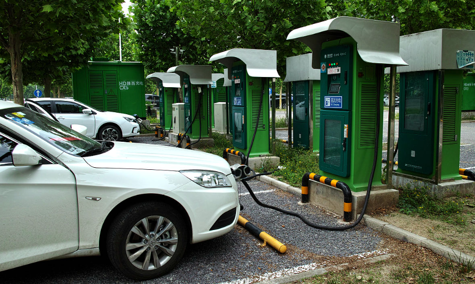
I formulate a planning framework in which electric vehicle charging demand is not treated as a single aggregate curve but as a spatially and temporally differentiated process generated by distinct travel and charging behaviors. The motivation is straightforward: uncoordinated electric vehicle charging can create sudden load surges that threaten distribution network security, while poorly located charging stations can concentrate demand on weak feeders, increase losses, accelerate equipment aging, and create voltage or current violations. I therefore combine travel-chain modeling, Monte Carlo simulation, road-network coupling, differentiated electrical safety constraints, and multi-objective optimization to select charging station locations and capacities. The framework is intended to provide a behavior-driven and network-aware basis for electric vehicle charging infrastructure planning.
I begin with the energy state of a vehicle. For a vehicle with battery capacity, energy consumption rate, and daily travel distance, the consumed energy, remaining energy, and state of charge after travel can be expressed as
$$E_{c}=E_{r}d$$
$$E_{rem}=C_{b}-E_{c}$$
$$SOC_{after}=\frac{E_{rem}}{C_{b}}$$
where the symbols denote consumed energy, energy consumption per unit distance, daily distance, remaining energy, battery capacity, and state of charge after travel. A charging event is generated when the remaining state of charge falls below a threshold or when the next trip requires a target state of charge. The required energy and charging duration are
$$E_{need}=\max\left(0,\left(SOC_{target}-SOC_{after}\right)C_{b}\right)$$
$$T_{ch}=\frac{E_{need}}{P_{ch}\eta_{ch}}$$
where the charging power and charging efficiency determine the duration. This event-based representation is important for electric vehicle charging analysis because it links travel distance, initial state of charge, charging threshold, and charging power within a single chain. I use this chain to generate charging events for private cars, taxis, and buses rather than applying one common probability distribution to all vehicles.
The temporal distribution of charging events is described by a mixture of normal distributions over multiple time windows:
$$f_{time}(t)=\sum_{i=1}^{N}\omega_{i}\frac{1}{\sqrt{2\pi}\sigma_{i}}\exp\left[-\frac{\left(t-\mu_{i}\right)^{2}}{2\sigma_{i}^{2}}\right]$$
where the weight, mean, and standard deviation of each window represent the relative probability and timing of electric vehicle charging for a given vehicle class. Initial state of charge and daily travel distance are represented by uniform distributions over class-specific intervals:
$$f_{SOC}(x)=\frac{1}{b-a},\quad x\in\left[a,b\right]$$
$$f_{s}(s)=\frac{1}{b-a},\quad s\in\left[a,b\right]$$
The charging probability at a given time is then obtained by combining the state-of-charge distribution and the time distribution. I allow up to two charging events per day for the main travel chain, so that
$$p(t)=\sum_{k=0}^{Q}f_{SOC}\left(I_{SOC}\right)f_{time}\left(t-k\right),\quad Q=2$$
This expression accumulates the probability that a charging event ends at time t after the k-th trip. The resulting electric vehicle charging load is generated by Monte Carlo sampling of vehicle class, initial state of charge, daily distance, charging window, charging power, and charging duration. The convergence criterion is based on the mean total load: after 1000 samples, the fluctuation of total charging load is less than one percent, so the simulation is considered sufficiently converged.
I differentiate three vehicle classes because their operating logic produces different temporal and spatial signatures. Private cars are the dominant group, with relatively stable daily distances and a strong preference for slow charging at home or at workplace parking. Taxis are high-frequency operating vehicles with urgent补能 needs; their behavior is modeled as a midday fast-charging event and a night slow-charging event, reflecting the trade-off between operating time and energy cost. Buses have large batteries and fixed schedules; they use high-power fast charging during daytime operating gaps and slow charging during long nighttime parking. These differences are essential for accurate electric vehicle charging load prediction.
| Vehicle class | Daily travel distance | Main charging mode | Typical charging windows | Spatial preference | Exclusivity and sharing |
|---|---|---|---|---|---|
| Private car | Moderate, approximately 30 to 80 km | Slow charging dominant, limited daytime slow charging | Before morning peak and late night | Residential area and workplace parking | Highly dedicated residential slow charging, with limited sharing of fast charging |
| Taxi | High, frequent daily operation | Fast and slow charging combination | Midday fast charging and night slow charging | Commercial nodes, transport hubs, residential surroundings | Strong sharing potential with private cars in commercial areas |
| Bus | Fixed route and depot-based | High-power fast charging and nighttime slow charging | Daytime schedule gaps and night parking | Industrial depots and dedicated terminals | Highly exclusive because of power demand, voltage level, and site requirements |
The spatial behavior of electric vehicle charging is organized around functional areas. In commercial areas, daytime passenger flow is dense and land cost is high. Private cars tend to shift charging to nighttime, while taxis dominate midday fast charging near transport hubs and commercial nodes. Private cars and taxis therefore exhibit substantial sharing potential in commercial areas, and differentiated pricing or time-of-use scheduling can improve fast-charging utilization. Buses generally do not produce commercial-area charging load unless a dedicated depot exists. In residential areas, private cars create the largest and most stable nighttime slow-charging base load, producing a valley-filling effect. Taxis may share surrounding fast or slow facilities after their shifts, whereas buses are largely absent because depots are separated from residential blocks. In industrial areas, the division is sharper: private cars use daytime workplace slow charging, taxis use opportunistic en-route charging, and buses require dedicated high-power charging because their power demand, voltage level, and scheduling constraints are incompatible with ordinary public charging.
| Functional area | Private car behavior | Taxi behavior | Bus behavior | Station design implication |
|---|---|---|---|---|
| Residential area | Nighttime slow charging base load; stable and large | Flexible nighttime or off-peak charging; shares fast chargers | Almost absent | Slow charging dominant with a small number of shared fast chargers |
| Commercial area | Limited daytime slow charging; high land cost discourages daytime charging | Main driver of midday fast charging; high turnover | Almost absent without a dedicated depot | Fast-charging sharing between taxis and private cars; pricing and scheduling are important |
| Industrial area | Daytime workplace slow charging | Random en-route charging; auxiliary service | Dedicated high-power fast charging and nighttime slow charging | Bus station planned independently; private and taxi stations as supporting facilities |
I construct a road-network coupling framework in which candidate nodes are mapped to a geographic coordinate system, and an origin-destination matrix records the distance between nodes. The shortest path is computed by Dijkstra’s algorithm, and the resulting travel trajectory determines where electric vehicle charging events occur. The origin-destination matrix has the form
$$P_{OD}=\left[0,\ d_{12},\ \ldots,\ d_{1,33};\ d_{21},\ 0,\ \ldots,\ d_{2,33};\ \ldots;\ d_{33,1},\ d_{33,2},\ \ldots,\ 0\right]$$
where each entry represents the road distance from one node to another. I couple the road layer to an IEEE 33-node distribution feeder. The nodes are assigned to residential, commercial, and industrial functional areas according to land-use characteristics. This coupling means that a vehicle trajectory determines the charging node, the charging node injects load into the distribution network, and the network response is evaluated by power flow. In this way, electric vehicle charging demand is not allocated by simple straight-line distance but by road-network accessibility and functional attraction.
The electrical safety constraint system is divided into hard constraints and soft constraints. Hard constraints protect the network from voltage collapse, line overload, and transformer overloading. Soft constraints guide the solution toward practical and balanced planning. I use a forward-backward sweep power flow to calculate node voltages and branch powers. The branch current constraint is
$$S_{ij}=\sqrt{3}V_{i}I_{ij}$$
$$I_{ij}\le z_{j}I_{ij}^{rated}$$
$$S_{ij}\le C_{ij}$$
where the current margin coefficient depends on the functional area. The voltage constraint is
$$V_{i}\ge V_{i,low}$$
where the lower limit is differentiated by area. The soft constraints include budget, station number, area coverage, line loading, and transformer capacity:
$$\sum_{i}C_{i}x_{i}\le B$$
$$N_{min}\le\sum_{i}x_{i}\le N_{max}$$
$$S_{node}(p)\le C_{dist}(p)z_{dist}(p)\eta_{dist}(p)$$
$$L_{j}\le L_{j}^{max}(z_{j})$$
$$S_{total}\le C_{sub}z_{sub}\eta_{sub}$$
The differentiated thresholds are summarized below. Residential areas use a stricter voltage lower limit because of sensitive household loads, while industrial areas allow a higher current margin because bus fast charging creates short-term high-power surges.
| Area type | Transformer capacity (kVA) | Voltage lower limit (p.u.) | Loading upper limit | Current margin coefficient |
|---|---|---|---|---|
| Residential | 500 | 0.93 | 70% | 1.0 |
| Commercial | 800 | 0.90 | 75% | 1.1 |
| Industrial | 1000 | 0.90 | 80% | 1.2 |
| Substation | 5000 | 0.95 | 85% | 1.0 |
I convert constraint violations into penalty terms so that the optimizer is driven toward the feasible region. The fitness is
$$F=F_{C}-P_{total}$$
where the comprehensive objective is reduced by the total penalty. The penalty components are grouped as
$$P_{hard}=P_{volt}+P_{amp}$$
$$P_{soft}=P_{load}+P_{sub}+P_{dist}$$
$$P_{fix}=P_{budget}+P_{count}+P_{coverage}$$
$$P_{total}=0.4P_{hard}+0.2P_{soft}+0.15P_{fix}$$
The voltage penalty and current penalty increase with the degree of violation, while the budget, station-number, and coverage penalties are binary when the corresponding limit is crossed. I also apply a budget-overrun discount factor in the economic objective so that a slightly over-budget but otherwise feasible plan is not discarded abruptly. The weighted penalty design is important because an electric vehicle charging plan that violates voltage or line limits cannot be accepted merely because it has low investment cost.
The penalty coefficients are calibrated by ablation. A weak-penalty scheme allows too many constraint violations and produces misleading fitness values. A strong-penalty scheme suppresses feasible exploration and makes the search overly conservative. The selected weighted scheme provides the best balance between constraint satisfaction and objective value, so I retain it in the final optimization.
| Penalty scheme | Constraint satisfaction | Objective value | Search behavior | Decision |
|---|---|---|---|---|
| Weak penalty, 0.5 times | Low to moderate | Apparently attractive but misleading | Accepts violated solutions too easily | Rejected |
| Current weighted penalty | High | Balanced | Maintains feasible exploration | Selected |
| Strong penalty, 2.0 times | Very high | Conservative | Suppresses useful exploration | Rejected |
The multi-objective function combines economic performance, road-network convenience, and distribution network operation quality:
$$\min F_{C}=w_{e}F_{e}+w_{r}F_{r}+w_{p}F_{p}$$
where the weights are determined by a combined entropy-weight and analytic-hierarchy process. The economic objective includes construction, equipment, land, and operation and maintenance costs:
$$F_{e}=\sum_{i}x_{i}\left(C_{co,i}+C_{land,i}+C_{op,i}\right)+\beta\sum_{i}\frac{S_{i}x_{i}}{M}+\chi B$$
where the normalized area score, station number, cost-efficiency factor, and budget-overrun factor adjust the cost comparison among candidate nodes. The road-network objective rewards accessibility, traffic flow, coverage, and uniform distribution:
$$F_{r}=w_{a}f_{accessibility}+w_{t}f_{traffic}+w_{c}f_{coverage}+w_{u}f_{uniformity}$$
The distribution network objective minimizes voltage deviation and line loading while improving load distribution uniformity:
$$F_{p}=w_{v}f_{v}+w_{l}f_{l}+w_{D}f_{D}$$
The weights are not selected arbitrarily. The entropy method provides objective information from generated feasible solutions, while the analytic-hierarchy process encodes planning priorities. The combined weights are obtained by linear fusion. The resulting weights are 0.240 for the economic objective, 0.497 for the distribution network objective, and 0.263 for the road-network objective. The high weight on the distribution network objective reflects the fact that high-power bus charging in industrial areas can create severe local voltage and capacity stress, so reliable supply is prioritized over land cost and road convenience.
| Objective | Analytic-hierarchy weight | Combined weight | Planning interpretation |
|---|---|---|---|
| Economic performance | 0.20 | 0.240 | Controls investment, land, equipment, and maintenance burden |
| Distribution network quality | 0.50 | 0.497 | Protects voltage, line capacity, transformer capacity, and load balance |
| Road-network convenience | 0.30 | 0.263 | Rewards accessibility, coverage, traffic attraction, and spatial uniformity |
I solve the siting and sizing problem with a genetic algorithm and particle swarm optimization. The genetic algorithm uses selection, crossover, and mutation to explore a combinatorial space, while particle swarm optimization updates individual and global best positions. The two algorithms are compared under the same penalty and objective structure. In this problem, the genetic algorithm shows stronger global search capability, so its result is used for the final electric vehicle charging station plan. The algorithm settings are summarized below.
| Algorithm | Population or particles | Maximum iterations | Crossover probability | Mutation probability | Role |
|---|---|---|---|---|---|
| Genetic algorithm | 100 | 200 | 0.8 | 0.1 | Global combinatorial search and final selection |
| Particle swarm optimization | 50 | 150 | Not applicable | Not applicable | Comparative benchmark |
The case study uses 1500 vehicles and a differentiated vehicle mix that reflects the functional characteristics of the road-network nodes. Each vehicle generates a complete charging-event chain in the Monte Carlo simulation. The simulation reaches convergence after 1000 samples, with total load fluctuation below one percent. The base voltage is 12.66 kV and the base power is 100 MVA. The economic parameters are differentiated by vehicle class because private cars, taxis, and buses use different charger powers and utilization patterns.
| Vehicle class | Normalization basis | Land cost coefficient | Equipment cost | Operation and maintenance cost |
|---|---|---|---|---|
| Private car | 8 kW per 10,000 currency units | 1.5 | 2 currency units per W for 7 kW slow charging | 300 currency units per charger per year |
| Taxi | 6 kW per 10,000 currency units | 2.0 | 0.7 currency units per W for 150 kW fast charging | 3000 currency units per charger per year |
| Bus | 9 kW per 10,000 currency units | 1.0 | 0.15 currency units per W for 45 kW slow charging and 0.8 currency units per W for 360 kW fast charging | 2000 to 8000 currency units per charger per year |
The optimized plan produces a spatially differentiated electric vehicle charging load. Industrial and residential areas accumulate higher total charging load than commercial areas. Commercial areas have the highest fast-charging load density because land is scarce and taxi turnover is high. Industrial areas have the highest peak because bus fast charging occurs during midday operating gaps. Residential areas show a stable all-day base load with a clear evening peak and a secondary midday peak caused by shared taxi fast charging. Commercial areas show two load surges, one at midday and one in the evening, driven by taxi operation. These patterns are consistent with the travel-chain assumptions and confirm that electric vehicle charging load should not be modeled as a single normalized profile.
| Area | Total charging load | Peak timing | Main driver | Network concern |
|---|---|---|---|---|
| Residential | High cumulative load | Evening peak with midday secondary peak | Private car nighttime slow charging and shared taxi fast charging | Voltage drop at feeder ends and transformer loading |
| Commercial | Moderate cumulative load | Midday and evening surges | Taxi fast charging and limited private car daytime charging | High load density and fast-charging current stress |
| Industrial | High cumulative load | Midday bus fast-charging peak and stable nighttime load | Bus daytime fast charging and nighttime slow charging | Short-term high-power surge and line capacity margin |
I evaluate the network impact by comparing node load before and after charging station integration. The load change at each node remains below 0.5 MW, which is acceptable for the feeder. The lowest voltage appears at the terminal node, following the typical voltage profile of a radial distribution feeder. The critical node is node 18, with a voltage of 0.9169 p.u. and a deviation of 5.51 percent. This value satisfies the functional-area voltage requirement and does not create a voltage violation. The industrial nodes have the highest loading rates, but they remain below the 80 percent upper limit. Therefore the optimized electric vehicle charging station plan satisfies the hard constraints while keeping the additional voltage drop within an acceptable range.
| Node | Minimum voltage (p.u.) | Voltage deviation (%) | Line capacity | Maximum loading rate (%) |
|---|---|---|---|---|
| 1 | 1.0000 | 0.00 | n/a | 0.00 |
| 2 | 0.9977 | 0.19 | 5.0 | 8.80 |
| 3 | 0.9835 | 1.10 | 4.0 | 5.88 |
| 4 | 0.9753 | 1.66 | 3.5 | 6.46 |
| 5 | 0.9675 | 2.20 | 3.0 | 7.67 |
| 6 | 0.9506 | 3.34 | 2.5 | 9.52 |
| 7 | 0.9460 | 3.70 | 2.0 | 21.80 |
| 8 | 0.9389 | 4.25 | 1.8 | 13.89 |
| 9 | 0.9296 | 4.98 | 1.6 | 22.25 |
| 10 | 0.9232 | 5.42 | 1.4 | 23.86 |
| 11 | 0.9226 | 5.45 | 1.2 | 15.50 |
| 12 | 0.9220 | 5.46 | 1.0 | 3.00 |
| 13 | 0.9198 | 5.48 | 0.9 | 4.67 |
| 14 | 0.9191 | 5.49 | 0.8 | 2.75 |
| 15 | 0.9185 | 5.50 | 0.7 | 3.71 |
| 16 | 0.9179 | 5.50 | 0.6 | 4.50 |
| 17 | 0.9171 | 5.51 | 0.5 | 6.00 |
| 18 | 0.9169 | 5.51 | 0.4 | 8.00 |
| 19 | 0.9968 | 0.20 | 2.0 | 2.20 |
| 20 | 0.9951 | 0.20 | 1.5 | 2.80 |
| 21 | 0.9948 | 0.20 | 1.0 | 4.60 |
| 22 | 0.9944 | 0.20 | 0.8 | 6.25 |
| 23 | 0.9818 | 1.17 | 1.8 | 13.56 |
| 24 | 0.9800 | 1.18 | 1.2 | 9.33 |
| 25 | 0.9791 | 1.18 | 0.9 | 14.22 |
| 26 | 0.9500 | 3.34 | 1.5 | 2.00 |
| 27 | 0.9491 | 3.35 | 1.0 | 3.40 |
| 28 | 0.9461 | 3.37 | 0.8 | 3.50 |
| 29 | 0.9439 | 3.38 | 0.6 | 9.33 |
| 30 | 0.9429 | 3.39 | 0.5 | 14.40 |
| 31 | 0.9413 | 3.40 | 0.4 | 16.00 |
| 32 | 0.9410 | 3.40 | 0.3 | 29.33 |
| 33 | 0.9409 | 3.40 | 0.3 | 10.67 |
The weighting method also requires validation because objective weights can hide weak constraint handling. A pure entropy-weight scheme and a pure analytic-hierarchy scheme both produce higher constraint violation in this problem, whereas the combined weighting scheme achieves the best balance between constraint satisfaction and objective value. This occurs because the entropy method reacts to solution dispersion but can misjudge indicators with large random fluctuation, while the analytic-hierarchy process captures planning preference but remains subjective. The combined method mitigates both weaknesses. I also test alternative weight schemes, including equal weights, economic priority, distribution priority, road priority, and pairwise priorities. The variation in individual objective values and the weighted comprehensive objective remains below seven percent, indicating that the selected plan is robust to reasonable weight changes.
| Weighting or sensitivity scheme | Main emphasis | Observed result | Planning conclusion |
|---|---|---|---|
| Entropy weight only | Data dispersion | Higher constraint violation | Not sufficient alone |
| Analytic hierarchy only | Expert priority | Higher constraint violation | Not sufficient alone |
| Combined weighting | Objective and subjective balance | Best balance between satisfaction and objective | Selected |
| Equal weights | No priority | Stable but less protective of network constraints | Benchmark only |
| Economic priority | Cost reduction | Lower cost but weaker network performance | Not preferred |
| Distribution priority | Network security | Strong constraint satisfaction with acceptable cost | Consistent with planning goal |
| Road priority | User convenience | Improved coverage but higher network stress | Needs constraint control |
The comparison between the genetic algorithm and particle swarm optimization confirms that the genetic algorithm has better global search capability for this mixed siting and sizing problem. Particle swarm optimization converges quickly in early iterations but becomes trapped in a local region, whereas the genetic algorithm maintains diversity and finds a better feasible plan. I therefore use the genetic algorithm result as the final electric vehicle charging station configuration. The final configuration respects the budget, station-number range, area coverage requirement, voltage limit, line current limit, transformer capacity limit, and loading-rate limit.
| Item | Setting or result |
|---|---|
| Total vehicles | 1500 |
| Monte Carlo samples | 1500 complete charging-event chains |
| Convergence check | Total load fluctuation below 1 percent after 1000 samples |
| Base voltage | 12.66 kV |
| Base power | 100 MVA |
| Power flow method | Forward-backward sweep |
| Road shortest path | Dijkstra algorithm |
| Optimization algorithms | Genetic algorithm and particle swarm optimization |
| Selected algorithm | Genetic algorithm |
| Maximum node load change | Below 0.5 MW |
| Critical voltage node | Node 18, 0.9169 p.u., 5.51 percent deviation |
| Hard constraint status | Satisfied |
The main methodological contribution is the coupling of behavior, space, and network security. The model captures the exclusivity and sharing characteristics of electric vehicle charging among private cars, taxis, and buses. It uses origin-destination travel and Dijkstra shortest paths instead of straight-line distance, so charging demand is assigned to realistic road-network nodes. It also introduces functional-area differentiated thresholds for voltage, transformer capacity, line loading, and current margin. These features make the electric vehicle charging station plan more defensible than a purely cost-based or distance-based allocation.
The penalty function is another important element. Hard constraints receive the highest weight because voltage and current violations directly affect network security. Soft constraints receive lower weights because they guide rather than prohibit. Fixed-count constraints use binary penalties because they represent planning logic rather than continuous physical limits. The weighted penalty is normalized to the same order of magnitude as the comprehensive objective, which prevents the optimizer from selecting an attractive but infeasible plan. This design is particularly relevant for electric vehicle charging planning because fast-charging stations can create local peaks that are invisible in annual energy balance but critical in short-term operation.
I also note that the framework is not tied to one specific feeder topology. The objective functions are computed at the node level, so the model can be transferred to a larger distribution system by replacing the network topology, line parameters, transformer data, and road-network geographic information. The computational complexity of the population-based algorithms depends mainly on the dimension of the decision vector rather than the number of stages. Therefore the method has methodological scalability for electric vehicle charging infrastructure planning in larger urban systems.
Several limitations remain. The road model does not yet include real-time traffic congestion, so travel time and charging arrival time are based on static shortest paths. A dynamic traffic assignment model could improve the temporal accuracy of electric vehicle charging demand. The network model does not explicitly include equipment aging, harmonic distortion, or transient voltage effects caused by ultra-fast charging. Future work can add aging factors, harmonic analysis, and power-quality constraints. Land price is also treated as a static coefficient, whereas actual urban land value changes over space and time. A spatiotemporal land-cost model could improve the economic objective. Finally, the charging stations are planned independently of distributed photovoltaic generation and battery storage. Coordinated planning of electric vehicle charging stations, photovoltaic generation, and storage could reduce peak network stress and improve renewable energy utilization.
In summary, I develop a behavior-driven, road-network-coupled, and network-security-constrained optimization model for electric vehicle charging station siting and sizing. The model represents private cars, taxis, and buses with differentiated travel and charging behavior, generates charging events by Monte Carlo simulation, assigns demand through an origin-destination road network, evaluates the distribution network by forward-backward sweep power flow, and optimizes economic performance, road-network convenience, and distribution network quality under differentiated functional-area constraints. The results show that the selected plan keeps node voltage and line loading within limits, limits node load change to an acceptable range, and provides a robust balance among cost, user convenience, and network security. The framework therefore offers a practical reference for electric vehicle charging infrastructure planning where spatiotemporal load distribution and electrical safety must be considered together.