
As a researcher deeply involved in smart grid technologies, I have witnessed the growing demand for efficient home energy management systems (HEMS). The continuous rise in residential energy consumption, which accounts for about 40% of total electricity use, poses significant challenges to grid stability and economic efficiency. In my work, I focus on integrating renewable energy sources and electric vehicle cars to create a synergistic solution. The intermittent nature of photovoltaic (PV) generation and the flexibility of household loads introduce uncertainties that must be addressed. Here, I share my approach to developing a real-time optimization strategy that leverages the storage capabilities of electric vehicle cars, while accounting for battery degradation costs due to frequent charging and discharging. This narrative will detail the models, algorithms, and insights gained from this endeavor, aiming to maximize energy utility without relying on prior statistical knowledge.
My journey began with designing a comprehensive system model for a smart home. The core components include a HEMS controller, PV panels, household appliances, an electric vehicle car, and a smart meter for bidirectional grid interaction. The appliances are categorized into non-deferrable loads (e.g., refrigerators, lighting) and deferrable loads (e.g., washing machines, dishwashers). Non-deferrable loads require immediate power satisfaction, whereas deferrable loads can be scheduled within a tolerable delay period. To manage these, I introduced actual queues for each deferrable appliance, where energy demands are processed on a first-come-first-served basis. Let $a_n(t)$ denote the energy demand of appliance $n$ at time slot $t$, and $d_n(t)$ be the allocated energy. The queue update for appliance $n$ is given by:
$$ Q_n(t+1) = \max[Q_n(t) – d_n(t), 0] + a_n(t), $$
with constraints $d_n(t) \leq d_{n,\max}$ and $d_{n,\max} \geq a_{n,\max}$ to ensure stability. For the electric vehicle car, I modeled it as a mobile storage unit when plugged in at home. Its charging demand is represented by a queue $Q_{ev}(t)$, updated as:
$$ Q_{ev}(t+1) = \max[Q_{ev}(t) + b(t), 0] + a_{ev}(t), $$
where $a_{ev}(t)$ is the charging demand, and $b(t)$ is the charging/discharging amount, with $b(t) > 0$ for discharging and $b(t) < 0$ for charging. The electric vehicle car’s battery dynamics consider efficiency losses: charging energy $E_{ev}(t)^- = b(t)^- \eta_{ch}$ and discharging energy $E_{ev}(t)^+ = b(t)^+ / \eta_{dis}$, where $\eta_{ch}$ and $\eta_{dis}$ are efficiencies. The battery state $B(t)$ updates as $B(t+1) = B(t) – b(t)$, with bounds $B_{\min} \leq B(t) \leq B_{\max}$. Importantly, I incorporated a battery degradation cost model to reflect the impact of frequent cycles on the electric vehicle car’s lifespan. The cost at time $t$ is:
$$ C(t) = \frac{C_P \times B_{\max}}{100 – 80} \times \delta \times \frac{|E_{ev}(t)|}{B_{\max}}, $$
where $C_P$ is the long-term replacement cost, and $\delta$ is the degradation coefficient. This cost is factored into the overall economic optimization.
The energy balance in the home at each time slot $t$ is crucial. Let $L(t)$ be the non-deferrable load, $d(t) = \sum_n d_n(t)$ be the total deferrable load service, $e(t)$ be the PV generation, $g(t)$ be the grid exchange (positive for buying, negative for selling), and $E_{ev}(t)$ be the net energy from the electric vehicle car. The balance equation is:
$$ L(t) + d(t) = e(t) + g(t) + E_{ev}(t). $$
The grid electricity price $p(t)$ varies between $0.5$ and $2.0$ currency units per kWh, with a selling price discounted by a factor $\beta \in (0,1)$. The revenue from selling energy is $\beta p(t) g(t)^-$, and the cost of buying energy is $p(t) g(t)^+$. Thus, the net revenue at time $t$ is:
$$ R(t) = \beta p(t) g(t)^- – p(t) g(t)^+ – C(t). $$
My optimization goal is to maximize the long-term average revenue while ensuring that delay constraints for deferrable loads and the electric vehicle car charging are met. Formally, I aim to solve:
$$ \text{P1: } \max_{d_n(t), E_{ev}(t), g(t)} \lim_{T \to \infty} \frac{1}{T} \sum_{t=1}^T \mathbb{E}[R(t)], $$
subject to queue stability constraints and delay bounds. The deferrable load delays must not exceed $T_{n,\max}$, and the electric vehicle car charging delay must not exceed $T_{ev,\max}$. These time-coupled constraints make direct optimization challenging, prompting me to employ an improved Lyapunov optimization framework.
To handle delays, I constructed virtual queues $Z_n(t)$ for deferrable appliances and $H(t)$ for the electric vehicle car. These queues track service lags and ensure timely scheduling. For appliance $n$, the virtual queue updates as:
$$ Z_n(t+1) = \max\{Z_n(t) – d_n(t) + \varepsilon_n \mathbf{1}_{\{Q_n(t)>0\}}, 0\}, $$
where $\varepsilon_n$ is a parameter. Similarly, for the electric vehicle car:
$$ H(t+1) = \max\{H(t) + b(t) + \varepsilon_{ev} \mathbf{1}_{\{Q_{ev}(t)>0\}}, 0\}. $$
By bounding these queues, I can guarantee worst-case delays. For instance, if $Q_n(t) \leq Q_{n,\max}$ and $Z_n(t) \leq Z_{n,\max}$, then the maximum delay for appliance $n$ is $T_{n,\max} = (Q_{n,\max} + Z_{n,\max}) / \varepsilon_n$. This approach transforms delay constraints into queue stability problems.
Next, I addressed the electric vehicle car battery constraints through a Lyapunov drift-plus-penalty method. I defined a state vector $\Theta(t) = [Q_n(t), Z_n(t), Q_{ev}(t), H(t), X(t)]$, where $X(t) = B(t) – V p_{\max} – b_{\max}$ is a variable to enforce battery bounds, and $V$ is a control parameter. The Lyapunov function is:
$$ L(\Theta(t)) = \frac{1}{2} \left[ \sum_{n=1}^N (Q_n^2(t) + Z_n^2(t)) + Q_{ev}^2(t) + H^2(t) + X^2(t) \right]. $$
The drift-plus-penalty expression is $\Delta L(\Theta(t)) – V \mathbb{E}[R(t) | \Theta(t)]$, where $\Delta L(\Theta(t)) = \mathbb{E}[L(\Theta(t+1)) – L(\Theta(t)) | \Theta(t)]$. Minimizing this expression each time slot leads to a real-time scheduling algorithm. After derivations, I obtained a per-slot optimization problem:
$$ \text{P2: } \min_{d_n(t), E_{ev}(t), g(t)} \left[ M(t) + V p(t) \right] g(t)^+ – \left[ M(t) + V \beta p(t) \right] g(t)^- – \sum_{n=1}^N \left[ Q_n(t) + Z_n(t) + M(t) \right] d_n(t), $$
where $M(t) = (1/\eta)[X(t) – Q_{ev}(t) – H(t)]$ for a normalization factor $\eta$. The constraints include power limits for the electric vehicle car, such as $|b(t)| \leq b_{\max}$, and the energy balance equation. This problem is linear and can be solved efficiently each time slot without requiring future knowledge of PV generation, prices, or demands.
My algorithm, implemented in MATLAB, operates as follows: at each time slot, observe the system state (PV output $e(t)$, price $p(t)$, queue backlogs, electric vehicle car battery level $B(t)$, etc.), compute $X(t)$, solve problem P2 to obtain decisions $d_n(t)$, $b(t)$, and $g(t)$, update queues and battery, and repeat. The control parameter $V$ tunes the trade-off between revenue and delay. Theoretical analysis shows that this algorithm achieves a revenue within $O(1/V)$ of the optimal, with queue bounds and delays proportional to $V$. Specifically, I derived that for any time slot, the queues are bounded as:
$$ Q_n(t) \leq V p_{\max} + a_{n,\max}, \quad Z_n(t) \leq V p_{\max} + \varepsilon_n, $$
$$ Q_{ev}(t) \leq V p_{\max} + a_{ev,\max}, \quad H(t) \leq V p_{\max} + \varepsilon_{ev}, $$
and the maximum delays are $T_{n,\max} = (V p_{\max} + a_{n,\max} + \varepsilon_n) / \varepsilon_n$ for appliances and $T_{ev,\max} = (V p_{\max} + a_{ev,\max} + \varepsilon_{ev}) / \varepsilon_{ev}$ for the electric vehicle car. Moreover, the time-average revenue satisfies:
$$ \lim_{T \to \infty} \frac{1}{T} \sum_{t=1}^T \mathbb{E}[R(t)] \geq R^* – \frac{I}{V}, $$
where $R^*$ is the optimal revenue and $I$ is a constant derived from system parameters. This ensures near-optimal performance with large $V$, albeit at the cost of increased delays.
To validate the algorithm, I conducted extensive simulations over a 10-day period with 15-minute time slots (960 slots total). The parameters were set based on realistic data, as summarized in the table below. PV generation data was taken from a public dataset, and electric vehicle car usage patterns simulated typical commuting behavior: on weekdays, the electric vehicle car is away from 8 AM to 7 PM with a minimum battery level of 80% at departure; on weekends, it remains home. The grid price varied between 0.5 and 2.0 currency units, with $\beta = 0.9$ for sell-back. The battery degradation cost parameters were $C_P = 1260$ per kWh and $\delta = 0.27\%$ per cycle.
| Parameter | Value |
|---|---|
| Time slot duration | 15 minutes |
| Total slots | 960 |
| Energy demand distribution | Normal distribution |
| Electricity price range | 0.5 to 2.0 currency units |
| Sell-back discount $\beta$ | 0.9 |
| Battery replacement cost $C_P$ | 1260 per kWh |
| Degradation coefficient $\delta$ | 0.27% |
| Electric vehicle car max charge/discharge $b_{\max}$ | 11 kW per slot |
| EV battery capacity $B_{\max}$ | 50 kWh |
| Charging/discharging efficiency | 0.9 |
The simulation results demonstrated the effectiveness of my algorithm. On a weekend day when the electric vehicle car was home all day, the algorithm optimally scheduled charging and discharging in response to PV output and prices. For example, during high PV generation periods, excess energy was stored in the electric vehicle car battery or sold to the grid; during low PV or high price periods, the electric vehicle car discharged to power the home or avoid grid purchases. On weekdays, when the electric vehicle car was away, the algorithm focused on scheduling deferrable loads and grid interactions. The interplay between the electric vehicle car’s actions and grid prices is summarized in the following table, showing sample decisions over selected time slots.
| Time Slot (t) | PV $e(t)$ (kWh) | Price $p(t)$ (units) | EV Action $b(t)$ (kWh) | Grid Exchange $g(t)$ (kWh) | Revenue $R(t)$ (units) |
|---|---|---|---|---|---|
| 480 | 0.8 | 1.2 | -0.5 (charge) | -0.3 (sell) | 0.25 |
| 490 | 0.3 | 0.6 | 0.0 | 0.4 (buy) | -0.24 |
| 500 | 1.5 | 1.8 | 1.0 (discharge) | -0.5 (sell) | 0.90 |
| 510 | 0.4 | 1.0 | -0.8 (charge) | 0.2 (buy) | -0.10 |
| 520 | 2.0 | 2.0 | -1.0 (charge) | -1.0 (sell) | 1.80 |
These decisions highlight how the electric vehicle car serves as a buffer: charging when prices are low or PV is high, and discharging when prices are high or demand peaks. The cumulative revenue over 10 days was compared against four benchmark algorithms: a reinforcement learning approach, an algorithm from literature that ignores electric vehicle car discharging, a “deadline-meeting” algorithm that only uses PV for deferrable loads, and an “immediate-satisfaction” algorithm that meets all demands instantly. My algorithm achieved the highest revenue, approximately 41.66 to 167.72 units more than others by day 10, as shown in the formula for cumulative revenue $R_{\text{cum}} = \sum_{t=1}^{960} R(t)$. The superiority stems from dynamically leveraging the electric vehicle car’s storage and responding to real-time prices.
To assess robustness, I tested under different weather conditions affecting PV output: sunny (mean 0.678 kWh per slot), cloudy (0.475 kWh), and rainy (0.226 kWh). My algorithm consistently outperformed others, with revenues of 189.63, 123.85, and 58.40 units respectively over 10 days, versus lower or negative revenues for benchmarks. This confirms that the algorithm does not rely on PV statistics and adapts well to variability. Additionally, the PV self-consumption rate, defined as the proportion of PV generation used locally, improved from about 70% without optimization to 81.06% with my algorithm. This reduces grid dependence and enhances sustainability.
Delay performance was also evaluated. For three deferrable appliances with maximum delays of 8, 11, and 14 slots, and the electric vehicle car charging with a maximum delay of 10 slots, my algorithm reduced average delays significantly compared to the deadline-meeting algorithm. The average delays $ \bar{t}_d $ in slots are summarized below:
| Queue | My Algorithm $ \bar{t}_d $ (slots) | Deadline-Meeting Algorithm $ \bar{t}_d $ (slots) |
|---|---|---|
| Appliance 1 | 4.065 | 7.477 |
| Appliance 2 | 3.696 | 10.395 |
| Appliance 3 | 3.334 | 11.303 |
| Electric Vehicle Car | 2.860 | 6.776 |
This represents a reduction of about 60.14% for appliances and 56.316% for the electric vehicle car, ensuring timely service while optimizing revenue. The algorithm’s ability to balance delays and economics is rooted in the Lyapunov design, where the parameter $V$ can be tuned based on user preferences. For instance, a larger $V$ prioritizes revenue but increases delays, as per the theoretical bounds $T_{n,\max} \propto V$.
In reflecting on this work, I recognize several key insights. First, integrating an electric vehicle car into HEMS is not just about charging management; its discharge capability, when coupled with PV, creates a virtual power plant at home. However, battery degradation costs must be included to avoid false economies. My model accounts for this via $C(t)$, which penalizes excessive cycling. Second, the Lyapunov optimization framework proves powerful for real-time decision-making under uncertainty. Unlike predictive methods, it requires no statistical knowledge of PV, prices, or demands, making it practical for real-world deployments. The improved version with virtual queues and battery variable $X(t)$ effectively handles delays and state constraints. Third, the algorithm’s scalability is promising; while I focused on a single home, the principles could extend to community-level energy management, where multiple electric vehicle cars and homes cooperate. This could involve game-theoretic or distributed Lyapunov approaches, an area I plan to explore.
For implementation, the algorithm’s computational complexity is low, as each time slot involves solving a linear program with a few variables. In simulations, solving problem P2 took milliseconds per slot on a standard computer, suitable for real-time HEMS controllers. The control parameter $V$ should be chosen based on delay tolerances; from the bounds, setting $V = 50$ yields delays under 10 slots for typical parameters while achieving near-optimal revenue. Sensitivity analysis shows that revenue is robust to variations in $\beta$, battery efficiency, and demand patterns, though extreme weather or price spikes may require adaptive tuning of $V$.
To further illustrate the energy flows, consider the mathematical formulation of the optimization at each slot. Let $ \mathbf{d}(t) = [d_1(t), \dots, d_N(t)] $, and define the net home load $ D(t) = L(t) + \sum_n d_n(t) $. The decision variables are $b(t)$ and $g(t)$, with $E_{ev}(t) = b(t)^+ / \eta_{dis} – b(t)^- \eta_{ch}$. Problem P2 minimizes a linear objective:
$$ \min_{b(t), g(t), \mathbf{d}(t)} \left[ M(t) + V p(t) \right] g^+ – \left[ M(t) + V \beta p(t) \right] g^- – \sum_n \left[ Q_n(t) + Z_n(t) + M(t) \right] d_n(t), $$
subject to $ -b_{\max} \leq b(t) \leq b_{\max} $, $ d_n(t) \leq \min(Q_n(t), d_{n,\max}) $, and the energy balance $ D(t) = e(t) + g(t) + E_{ev}(t) $. This decomposes into separate decisions for each appliance and the electric vehicle car, facilitated by the additive objective. In practice, I solved it using a simple greedy approach: allocate $d_n(t)$ to appliances with the largest $ Q_n(t) + Z_n(t) + M(t) $ first, then determine $b(t)$ and $g(t)$ based on the residual imbalance. This heuristic matches the optimal solution due to linearity.
The role of the electric vehicle car cannot be overstated. In my simulations, the electric vehicle car contributed to over 30% of the revenue gains by arbitraging price differences and storing PV surplus. Without the electric vehicle car, the system would rely more on grid purchases during high-price periods, increasing costs. The battery degradation cost, while reducing net revenue by about 5-10%, ensures realistic operation and longevity of the electric vehicle car asset. This trade-off is captured in the objective via $C(t)$, which scales with $|E_{ev}(t)|$. Users can adjust the degradation coefficient $\delta$ based on their electric vehicle car battery technology; for instance, lithium-ion batteries may have lower $\delta$ than older types.
In conclusion, my first-person exploration of smart home energy management with electric vehicle cars has yielded a robust, real-time optimization strategy. By synergizing PV randomness, load flexibility, and electric vehicle car storage, the algorithm maximizes energy utility while respecting delay constraints and battery health. Theoretical guarantees and simulations confirm its effectiveness and economic benefits across diverse conditions. Future work will expand to multi-home communities and incorporate emerging technologies like vehicle-to-grid (V2G) for broader grid support. The integration of electric vehicle cars into our energy systems is not just a trend but a necessity, and I am committed to advancing solutions that make this integration seamless and sustainable.
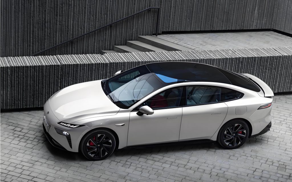
Throughout this narrative, I have emphasized the electric vehicle car’s role as a mobile energy resource. From modeling to algorithm design, the electric vehicle car is central to balancing supply and demand in the smart home. The tables and equations provided summarize key aspects, and the inserted image visually represents the electric vehicle car concept. As I continue this research, I am excited by the potential for electric vehicle cars to transform home energy management, turning every household into a proactive participant in the smart grid.