
In my research, I focused on a central challenge in modern electric mobility: the consistency of cells inside an EV battery pack. The growing deployment of battery-powered vehicles requires high-voltage and high-capacity storage systems; however, the capacity of a single lithium-ion cell is not sufficient for traction applications. Therefore, many cells must be connected in series and parallel to form a complete EV battery pack. The unavoidable initial differences among those cells, together with the operating environment, cause the internal states of the cells to diverge further as the pack is cycled. Over time, this divergence leads to premature failure of the whole EV battery pack and severe material waste. In this context, the goal of my work was to develop a fast, non-destructive and reliable method for sorting cells before they are assembled into an EV battery pack.
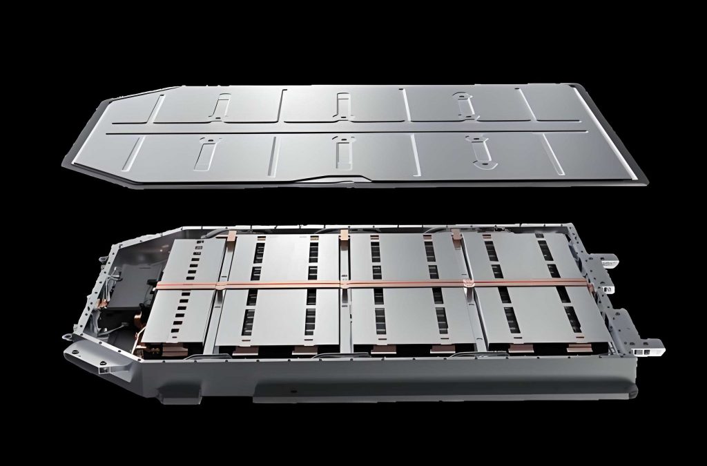
Traditional battery sorting methods usually measure external characteristics such as open-circuit voltage, internal resistance, static capacity and self-discharge rate. These measurements are useful, but they only indirectly capture the internal condition of the active materials, the electrolyte conductivity and the solid-electrolyte interphase quality. For an EV battery pack, the external parameters are not sufficient to guarantee that the internal states of the cells are matched. A battery cell is a complex electrochemical system; two cells with the same capacity can have completely different internal electrode structures and different aging states. Therefore, I decided to use electrochemical impedance spectroscopy, or EIS, to probe the internal properties directly. EIS is a small-signal frequency-domain technique that can reveal the electrode kinetics, diffusion behavior and interfacial properties inside a cell without damaging it. This principle was the foundation of the multi-spectral method that I proposed for EV battery pack cell sorting.
1. Background and Motivation for Battery Consistency
The idea of battery consistency is related to the classic “barrel effect”: the performance of an EV battery pack is governed by the weakest cell in the pack. If one cell has a lower capacity or a higher internal resistance, it will reach the discharge cut-off voltage earlier than the others. During charging, the same cell will reach the upper voltage limit earlier. As a result, the control system must stop charging or discharging before the remaining cells have been fully used. This creates an apparent capacity loss in the whole EV battery pack and accelerates the degradation of the weakest cell.
There are several types of consistency that matter in an EV battery pack. The first is voltage consistency. In a parallel-connected string, a low-voltage cell will be charged by the other parallel cells, causing parasitic current loops and unwanted heat generation. The second is capacity consistency. If cells in a series string have different capacities, the low-capacity cell will become over-discharged while the high-capacity cells are still delivering useful energy. The third is resistance consistency. In a series-connected EV battery pack, the cell with the highest internal resistance dissipates more heat and develops a larger voltage drop during high-current operation. In a parallel-connected string, the current is inversely proportional to the internal resistance, so cells with different resistances operate at different charge and discharge rates. All of these consistency issues are strongly coupled, and they can only be mitigated, not completely eliminated, by sorting cells before assembly.
Table 1 summarizes the main performance parameters of different battery chemistries historically used for traction. Lithium iron phosphate, LiFePO4, is especially promising for EV battery pack applications because of its long cycle life, thermal stability, and low material cost. The operating voltage is about 3.6 V, and its energy density is sufficient for many electric vehicle applications. In my study, I selected commercial 18650 LiFePO4 cells as the research object because they are widely used in small-format EV battery pack designs and especially in electric tool applications.
| Battery type | Voltage (V) | Specific energy (Wh/kg) | Energy density (Wh/L) | Memory effect | Cycle life at 80% DOD |
|---|---|---|---|---|---|
| VRLA | 2.0 | 35 | 80 | No | 400 |
| Cd-Ni | 1.2 | 45 | 160 | Yes | 500–1000 |
| MH-Ni | 1.2 | 70 | 240 | Yes | 500–800 |
| LiB | 3.6 | 125 | 300 | No | 600–1000 |
| PLiB | 3.6 | 200 | 300 | No | 600–1000 |
| LiFePO4 | 3.3 | 90–110 | 220 | No | 1000–2000 |
The initial inconsistency among cells originates from two broad sources. The first source is manufacturing. During electrode coating, roll pressing and electrolyte filling, minor differences in active material loading, electrode thickness, porosity and activation level are inevitable. The second source is operational use. Temperature gradients, vibration, charge/discharge history and self-discharge rates all differ among cells inside an EV battery pack. These differences cause the internal resistance and capacity to diverge progressively. Therefore, my research aimed to identify a practical sorting criterion that is based on the internal electrochemical state rather than only the external behavior of the cell.
2. Electrochemical Impedance Spectroscopy and Equivalent Circuits
EIS is based on the response of an electrochemical system to a small sinusoidal perturbation. For a stable linear system, if the input signal is a small sinusoidal voltage or current with angular frequency \(\omega\), the output signal is also sinusoidal with the same frequency but with a different amplitude and phase. The transfer function in the frequency domain is called the impedance:
$$Z(\omega) = \frac{V(\omega)}{I(\omega)}.$$
By measuring the impedance at a series of frequencies, I obtained a complex impedance spectrum. The Nyquist plot, which plots \(-Z”\) against \(Z’\), is the most common representation of EIS data. For a pure resistor \(R\), the impedance is real and independent of frequency:
$$Z_R = R,\quad Z_R’ = R,\quad Z_R” = 0.$$
For a pure capacitor \(C\), the impedance is purely imaginary:
$$Z_C = \frac{1}{j\omega C},\quad Z_C’ = 0,\quad Z_C” = -\frac{1}{\omega C}.$$
In a real electrochemical cell, the electrode-electrolyte interface cannot be modeled by an ideal capacitor. The roughness and porosity of the electrode surface cause the interfacial capacitance to behave as a constant phase element, denoted by \(Q\). The impedance of a constant phase element is:
$$Z_Q = \frac{1}{Y_0 (j\omega)^n},$$
where \(Y_0\) is the admittance coefficient and \(n\) is an exponent between 0 and 1. When \(n = 1\), the element behaves as a pure capacitor; when \(n = 0\), it behaves as a pure resistor. The phase angle of the constant phase element is \(n\pi/2\), which explains why the impedance arcs in real battery measurements are often depressed semicircles rather than perfect semicircles.
2.1 Simple composite elements
An equivalent circuit is assembled from resistors, capacitors, inductors and constant phase elements. The configuration of these elements must have a physical meaning in terms of the electrode reactions, the double-layer capacitance, the electrolyte resistance and the diffusion process. The simplest composite element is the series combination of a resistor and a capacitor:
$$Z = R + \frac{1}{j\omega C} = R – \frac{j}{\omega C}.$$
In the Nyquist plot, this series combination appears as a vertical line with zero real part at high frequency and asymptotically approaching the real axis at high frequency. However, this is not observed in LiFePO4 cells.
A more realistic composite element is the parallel combination of a resistor and a capacitor, which represents a single electrode interface. The impedance is:
$$Z = \frac{R}{1 + j\omega RC}.$$
Separating the real and imaginary parts gives:
$$Z’ = \frac{R}{1 + (\omega RC)^2},\quad Z” = -\frac{\omega R^2 C}{1 + (\omega RC)^2}.$$
After algebraic manipulation, one can show that the Nyquist plot is a semicircle:
$$\left(Z’ – \frac{R}{2}\right)^2 + (Z”)^2 = \left(\frac{R}{2}\right)^2.$$
For a real battery electrode, the constant phase element should be used instead of the ideal capacitor. The impedance of a resistor \(R\) in parallel with a constant phase element \(Q\) is:
$$Z = \frac{R}{1 + R Y_0 (j\omega)^n}.$$
The corresponding Nyquist plot is a depressed arc with its center below the real axis when \(0 < n < 1\). The equation of this arc can be written as:
$$\left(Z’ – \frac{R}{2}\right)^2 + \left(Z” – \frac{R}{2}\cot\frac{n\pi}{2}\right)^2 = \left(\frac{R}{2\sin(n\pi/2)}\right)^2.$$
This depressed semicircle is exactly what I observed for LiFePO4 cells. Therefore, I used constant phase elements rather than pure capacitors in the equivalent circuit of the EV battery pack cells.
2.2 Warburg diffusion impedance
At low frequencies, the impedance of a battery often reflects diffusion of lithium ions in the solid electrode particles. The so-called Warburg impedance represents semi-infinite linear diffusion and has the following expression:
$$Z_W = \frac{\sigma}{\sqrt{\omega}} (1 – j),$$
where \(\sigma\) is the Warburg coefficient. This impedance has a phase angle of \(\pi/4\), so its Nyquist line has a slope of unity. In my experiments, the low-frequency branch of the LiFePO4 impedance spectrum was not exactly a 45-degree line. Instead, the slope depended on the cell state and the electrode microstructure. This observation confirmed that a generalized constant phase element is more suitable than a pure Warburg element in the equivalent circuit for LiFePO4 cells.
3. Experimental Design and EIS Data Collection
All EIS measurements in my study were made with a CHI650D electrochemical workstation. The instrument is capable of measuring impedance from 100 kHz down to very low frequencies and can operate in two-, three-, or four-electrode modes. Four-electrode measurement is particularly important for batteries because it eliminates the influence of cable and contact resistance. For the cycle-life tests, I used a battery performance tester that can independently control the charging and discharging of each cell. The batteries were commercial 18650 LiFePO4 cells manufactured for electric vehicles and power tools. All cells were fresh, activated and unused before the experiments.
My objective was to build a large database of EIS spectra from LiFePO4 cells under different conditions. First, I measured the EIS of every cell in a fully charged state. Second, I measured the EIS at different states of charge during discharge, namely 25%, 50%, 75% and 0% remaining capacity. Third, I measured the impedance during charging at the same intermediate states. Finally, I selected a subset of cells for extended life cycling. After every 50 cycles, I measured the EIS again until the cell capacity fell below 80% of its rated value.
The database was important because an EV battery pack should be assembled from cells whose internal states are as close as possible. A sorting method based on only one voltage or capacity measurement cannot guarantee the internal state matching of the cells. The EIS database allowed me to identify which impedance parameters were stable and which were sensitive to aging.
4. Hough Transform for EIS Pattern Recognition
Before building an equivalent circuit, I needed a systematic method to analyze the shape of the measured EIS spectra. The Nyquist plots for LiFePO4 cells display a high-frequency arc and a low-frequency tail. Some authors describe the tail as a straight line, while others describe it as part of a very large semicircle. To resolve this ambiguity, I applied a Hough transform algorithm to recognize the circle-like and line-like features of the impedance spectra.
The Hough transform maps image-space points to parameter-space curves. A straight line in the image space can be represented as:
$$r = x\cos\theta + y\sin\theta.$$
Each point \((x, y)\) in the image corresponds to a sinusoidal curve in the \((r, \theta)\) parameter space. If several points lie on the same straight line, their parameter-space curves intersect at a common point. A circle can be represented as:
$$(x – a)^2 + (y – b)^2 = r^2,$$
where \((a, b)\) is the center and \(r\) is the radius. The Hough transform accumulates votes in the three-dimensional parameter space \((a, b, r)\), and the maximum votes identify the most probable circle in the image. I used this method to analyze the EIS spectra in the database. The flow of the algorithm was straightforward: extract the Nyquist plot, detect the edges, compute the Hough transform, identify the dominant circle, and record the center and radius. For each spectrum, I also performed a second recognition after removing the low-frequency part to determine whether the low-frequency branch more closely resembled a line or a large arc.
Table 2 summarizes the recognition results for 100 LiFePO4 cells. The test was carried out twice for each cell, so 200 recognition results were collected. I defined a low-frequency branch as a straight line if the deviation from a straight line was less than 5% or if the fitted radius of the largest arc was greater than 0.1. Under this rule, about 96% of the LiFePO4 spectra show a single semicircular arc plus a low-frequency straight line. This result is very different from the conventional double-semicircle spectra of nickel-metal hydride or cobalt-based lithium cells.
| Recognition criterion | First measurement | Second measurement |
|---|---|---|
| Low-frequency branch recognized as line | 95 | 97 |
| Low-frequency branch recognized as semicircle | 5 | 3 |
| High-frequency arc center above real axis | 2 | 2 |
| High-frequency arc center on real axis | 1 | 0 |
| High-frequency arc center below real axis | 97 | 98 |
Based on these results, I concluded that the high-frequency arc of LiFePO4 cells is a depressed semicircle, which is consistent with a resistor in parallel with a constant phase element. The low-frequency branch is a line with a slope that is not necessarily 45 degrees, so a constant phase element is more general than a Warburg element. The equivalent circuit that naturally emerged from the Hough recognition was the series combination of an ohmic resistance \(R_s\), a parallel \(R_1Q_1\) element for one electrode interface, and a parallel \(R_2Q_2\) element for the other interface. I write this circuit compactly as R(QR)(QR) or equivalently \(R_s (R_1 Q_1)(R_2 Q_2)\).
5. Equivalent Circuit Model for the LiFePO4 Cell
The equivalent circuit for a LiFePO4 cell in my model is shown in simplified form as \(R_s (R_1 Q_1)(R_2 Q_2)\). The ohmic resistance \(R_s\) includes the electrolyte resistance, the separator resistance and the contact resistance. The first parallel branch represents the positive electrode interface, and the second parallel branch represents the negative electrode interface. In some measured spectra, a small inductive tail appears at frequencies above 1 kHz. This inductive effect is caused by the porous structure and the non-uniform current distribution inside the cell, and it is usually negligible for EV battery pack operating frequencies. In the practical sorting model, I ignored the inductance in order to simplify the fitting procedure.
To verify the model, I fitted the measured EIS spectra using ZSimpWin software. The equivalent circuit was denoted as RQ(RQ) in the software. Table 3 shows a typical fitting result for a fresh LiFePO4 cell. The fitting errors for all parameters were small, and the chi-square quality was satisfactory.
| Parameter | Start value | Fitted value | Relative error (%) |
|---|---|---|---|
| \(R_1\) (Ω) | 0.03056 | 0.03056 | 0.6815 |
| \(Y_{01}\) | 195.8 | 195.9 | 2.641 |
| \(n_1\) | 0.8 | 0.4389 | 1.565 |
| \(R_2\) (Ω) | 0.01 | 0.008784 | 3.703 |
| \(Y_{02}\) | 1.989 | 1.989 | 12.82 |
| \(n_2\) | 0.8 | 0.7191 | 3.887 |
The fitted curve overlapped with the measured data very well, which confirmed that the \(R_s(R_1Q_1)(R_2Q_2)\) model represents the electrochemical behavior of the LiFePO4 cell accurately. For comparison, I also tried the classical model \(R_s(R_1C_1)(R_2C_2)\), which uses pure capacitors. This model is commonly used for cobalt-based lithium-ion cells, but it could not reproduce the measured LiFePO4 impedance spectrum correctly. The arcs were too symmetrical and the low-frequency tail had the wrong slope. I also tested a model containing a Warburg element, \(R_s(Q(RW))\). This model performed better at high and medium frequencies, but at low frequencies it was too restrictive because the Warburg impedance always gives a 45-degree line. Therefore, the constant phase element model was chosen as the final equivalent circuit for the LiFePO4 cell in an EV battery pack.
6. Effect of State of Charge on EIS
One important question for a practical sorting method is whether the state of charge, or SOC, affects the impedance spectrum. I measured the EIS of the same cell in two states: fully charged at SOC = 100% and fully discharged at SOC = 0%. The results showed that the impedance of the discharged cell was significantly larger than that of the charged cell. The depressed semicircle of the discharged cell was also more pronounced. This is because a fully discharged LiFePO4 electrode has lower electronic conductivity and a different lithium concentration at the electrode surface.
For sorting an EV battery pack, the state of charge must be the same for every measured cell. If the cells are not at the same SOC, the difference in the impedance spectra will be caused by SOC rather than by the internal state of the cells. I therefore decided to perform all sorting measurements in the fully charged state. This is convenient for production because cells are usually charged before delivery. It also avoids the risk of accidentally selecting a severely aged cell that might appear normal in the discharged state.
7. Multi-Spectral Method for Fast Sorting
The full EIS measurement is accurate but time-consuming. A complete frequency sweep from 100 kHz down to 0.01 Hz may take more than ten minutes per cell. For mass production of an EV battery pack, this is not acceptable. My solution was to propose a multi-spectral method based on the EIS equivalent circuit. Instead of measuring the entire impedance spectrum, I selected a small number of characteristic frequencies, measured the impedance at those frequencies, and then used a least-squares fitting algorithm to reconstruct the equivalent-circuit parameters. This method gives almost the same information as a full EIS scan but with a huge reduction in measurement time and complexity.
The key is to select the frequency points carefully. The EIS spectrum of a LiFePO4 cell can be divided into three regions: the high-frequency inductive tail, the medium-frequency depressed semicircle and the low-frequency straight tail. For practical sorting, I ignored the very high frequency inductive tail and focused on the frequency range from 0.5 Hz to 500 Hz. Within this range, I selected five frequency points:
| Point | Frequency (Hz) | Region |
|---|---|---|
| 1 | 0.5 | Low-frequency linear tail |
| 2 | 5 | Lower transition region |
| 3 | 20 | Middle of the arc |
| 4 | 50 | Upper transition region |
| 5 | 500 | High-frequency tail |
These frequency points were not chosen uniformly along the frequency axis. Instead, they were distributed according to the characteristic shape of the EIS curve. I determined the transition frequencies from the statistical analysis of the 100-cell database: the lower transition was near 5 Hz and the upper transition was near 50 Hz. The five selected points therefore cover the linear branch, the lower transition, the arc, the upper transition and the high-frequency region. This non-uniform distribution ensures that the reconstructed spectrum is representative of the complete EIS curve.
To test the reconstruction quality, I first fitted the full EIS spectrum using the equivalent circuit model. Then I used only the impedance values at the selected frequencies and fitted a fifth-degree polynomial to the complex impedance data. The polynomial model can be written as:
$$Z'(\omega) = a_0 + a_1 \log \omega + a_2 (\log \omega)^2 + a_3 (\log \omega)^3 + a_4 (\log \omega)^4 + a_5 (\log \omega)^5,$$
$$Z”(\omega) = b_0 + b_1 \log \omega + b_2 (\log \omega)^2 + b_3 (\log \omega)^3 + b_4 (\log \omega)^4 + b_5 (\log \omega)^5.$$
The least-squares method minimizes the sum of the squares of the residuals between the measured and fitted values. I also tested a ten-point version of the method in which the selected frequencies were more densely spaced. Table 4 compares the fitted equivalent-circuit parameters for the standard full-spectrum model, the ten-point method and the five-point method.
| Parameter | Full EIS model | Ten-point fitting | Five-point fitting |
|---|---|---|---|
| \(R_s\) (Ω) | 0.02586 | 0.02567 | 0.02564 |
| \(Y_{01}\) | 186.1 | 160.6 | 145.6 |
| \(n_1\) | 0.5612 | 0.5414 | 0.4943 |
| \(R_2\) (Ω) | 0.008568 | 0.008684 | 0.007269 |
| \(Y_{02}\) | 2.102 | 2.133 | 2.303 |
| \(n_2\) | 0.7107 | 0.6581 | 0.6994 |
The differences between the ten-point method and the five-point method were small. In several parameters, the fitting errors were within a few percent. This result was expected because the EIS curve of a LiFePO4 cell is smooth and continuous, so a small number of carefully placed frequency points can capture its shape almost as well as a large number of points. The five-point method therefore became the core of my proposed sorting procedure for EV battery pack cells.
8. Consistency Criterion and Statistical Analysis
In order to compare the consistency of cells in an EV battery pack, I used a statistical measure of dispersion. The standard deviation of a set of parameters is defined as:
$$\sigma = \sqrt{\frac{\sum_{i=1}^{n} (X_i – \bar{X})^2}{n}},$$
where \(X_i\) is the value of the \(i\)-th cell parameter, \(\bar{X}\) is the arithmetic mean, and \(n\) is the number of cells. The standard deviation is sensitive to extreme values and reflects the overall scatter of the data. I also used a dimensionless consistency coefficient:
$$K = \frac{\sigma}{\bar{X}}.$$
A smaller value of \(K\) indicates better consistency. In my experiments, I used this coefficient to evaluate both the EIS fitting parameters and the operating voltages of the battery packs during discharge.
I designed a validation experiment with two groups of eight cells connected in series. In the first group, the cells were sorted according to their EIS equivalent-circuit parameters. In the second group, the cells were sorted according to the conventional capacity and internal-resistance criteria. Both EV battery pack groups were discharged at 5 A, and the voltage of each cell was recorded. Table 5 shows the average pack voltage and the consistency coefficient at different discharge times for both groups.
| Discharge time (min) | EIS-sorted avg. voltage (V) | EIS-sorted \(K\) | Conventional sorted avg. voltage (V) | Conventional sorted \(K\) |
|---|---|---|---|---|
| 30 | 3.63 | 0.004 | 3.64 | 0.005 |
| 60 | 3.60 | 0.005 | 3.61 | 0.009 |
| 80 | 3.58 | 0.008 | 3.57 | 0.007 |
| 100 | 3.59 | 0.010 | 3.56 | 0.011 |
| 120 | 3.55 | 0.014 | 3.51 | 0.017 |
| 130 | 3.49 | 0.013 | 3.38 | 0.023 |
| 140 | 3.30 | 0.045 | 3.19 | 0.086 |
| 150 | 3.13 | 0.067 | 3.06 | 0.104 |
At the beginning of discharge, the two groups behaved similarly. As the discharge progressed, the conventional group showed a much larger voltage dispersion, especially after 120 minutes. The EIS-sorted group maintained a lower consistency coefficient and therefore a more uniform voltage distribution. This demonstrates that cells with matching internal electrochemical parameters perform more consistently in an EV battery pack under deep discharge conditions.
9. Practical Validation of the Five-Point Multi-Spectral Method
After verifying the five-point reconstruction in simulation, I performed a real sorting test. I prepared 80 fresh LiFePO4 cells with a nominal capacity of 1000 mAh and divided them into four groups of 20 cells. From each group, I selected eight cells to form an EV battery pack. The four packs were sorted by four different methods:
- capacity sorting only,
- capacity plus internal resistance sorting,
- five-point multi-spectral EIS sorting,
- ten-point multi-spectral EIS sorting.
All cells were first fully charged using a three-stage charging protocol to 4.2 V and then rested for two hours. The multi-spectral measurement was performed in the fully charged state with a four-wire connection. The five measurement frequencies were 0.5 Hz, 5 Hz, 20 Hz, 50 Hz and 500 Hz. The measured impedance values were used to reconstruct the equivalent-circuit parameters, and the cells were sorted according to those parameters. Then the packs were cycled under different discharge currents and depths in order to simulate the realistic operating conditions of an EV battery pack.
I defined the lifetime of the pack as the number of cycles until the measured capacity dropped to 80% of the rated initial capacity. The results are shown in Table 6.
| Sorting method | Initial capacity (mAh) | Cut-off capacity (mAh) | Cycle life |
|---|---|---|---|
| Capacity only | 8027.4 | 6401.6 | 142 |
| Capacity + internal resistance | 8015.8 | 6400.8 | 195 |
| Five-point multi-spectral method | 8034.2 | 6402.1 | 309 |
| Ten-point multi-spectral method | 8022.6 | 6401.5 | 326 |
The multi-spectral method significantly improved the cycle life of the EV battery pack compared with the conventional methods. The five-point method achieved a cycle life of 309 cycles, while the capacity-only method achieved only 142 cycles. The ten-point method improved the cycle life slightly to 326 cycles, but it required twice as many measurements. In a mass-production environment, the five-point method offers the best trade-off between measurement effort and sorting quality.
During the tests, I also observed that the initial capacities of all four packs were very similar. The difference was much smaller than the difference in cycle life. This confirms that the conventional capacity measurement cannot predict the long-term consistency of an EV battery pack. The internal impedance parameters, on the other hand, capture the interface quality and the diffusion properties that determine how uniformly the cells age.
10. Advantages and Practical Considerations
One of the most important advantages of the multi-spectral method is that it is non-destructive. The measurement is performed with a small sinusoidal perturbation, usually less than 10 mV, so the cell is not damaged and its state of charge is not significantly changed. The method is also fast. A full EIS scan can take more than ten minutes, while a five-point measurement can be completed in less than two minutes. This makes it suitable for inline sorting in battery production lines and for maintenance testing of an EV battery pack in service.
Another advantage is that the method is energy-saving. Conventional capacity sorting requires one or more complete charge-discharge cycles, which consume a large amount of energy and produce heat. The multi-spectral method requires only a small amount of electrical energy per measurement. For a battery manufacturer that processes thousands of cells per day, the energy saving is significant.
The frequency point of 500 Hz deserves a comment. In the final design of a dedicated sorting instrument, generating a precise 500 Hz test signal may require more expensive electronics than a lower frequency. My additional tests showed that reducing the highest frequency to 200–300 Hz does not significantly increase the sorting error if the other four frequency points are kept unchanged. Therefore, in a low-cost instrument, the highest frequency can be lowered without compromising the basic consistency of the EV battery pack sorting.
The multi-spectral method is not limited to LiFePO4 chemistry. The same principle can be applied to other lithium-ion chemistries, nickel-metal hydride batteries and lead-acid batteries. For each chemistry, the equivalent circuit and the frequency points must be adjusted according to the characteristic impedance spectrum. In my work, I focused on LiFePO4 because it is currently one of the most important materials in the electric vehicle market. The methodology, however, is general and can be adapted to other types of EV battery pack cells.
11. Conclusion
In my research, I proposed and validated a multi-spectral method for the consistency sorting of LiFePO4 cells intended for EV battery pack assembly. The main achievements of my work can be summarized as follows.
First, I established a complete EIS database for commercial LiFePO4 cells under different states of charge and states of health. Using the Hough transform, I statistically analyzed the impedance spectra and found that the low-frequency branch is usually a non-ideal straight line and the high-frequency arc is a depressed semicircle. This led to the equivalent circuit \(R_s(R_1Q_1)(R_2Q_2)\). The model was verified by nonlinear least-squares fitting and comparison with alternative circuit models.
Second, I demonstrated that the equivalent-circuit parameters can be used as sorting indicators. In a series-connected pack, cells sorted by EIS parameters showed a smaller voltage dispersion during deep discharge than cells sorted by conventional capacity and internal resistance. This is because the EIS parameters are directly related to the cell’s internal electrode structure, electrolyte condition and interfacial quality.
Third, I developed the five-point multi-spectral measurement procedure. The selected frequencies are 0.5 Hz, 5 Hz, 20 Hz, 50 Hz and 500 Hz. These five points were chosen according to the characteristic geometry of the EIS spectrum, not by uniform frequency spacing. With these five measurement points, a fifth-degree least-squares polynomial can reconstruct the impedance spectrum and the equivalent-circuit parameters with sufficient accuracy for battery sorting.
Fourth, a real pack-aging experiment confirmed that the five-point method increases the lifetime of the assembled EV battery pack dramatically. The cycle life improved from 142 cycles with capacity-only sorting to 309 cycles with the five-point method. The marginal improvement of the ten-point method was not large enough to justify the extra measurement time.
The multi-spectral method provides a practical bridge between the scientific richness of electrochemical impedance spectroscopy and the high-throughput demands of industrial EV battery pack manufacturing. It is fast, non-destructive, energy-saving and robust. Although the method was developed for LiFePO4 cells, the same framework can be extended to other battery chemistries. In the future, I believe that impedance-based sorting will become a standard step in the production of high-quality EV battery pack systems, helping to reduce cost, improve reliability and extend the lifetime of electric vehicles.