
My research focuses on the safety and reliability of traction battery packs. I have spent years analyzing real-world operating data collected from electric vehicles. The growing adoption of electric vehicles has brought great opportunities, but also challenges. Among these challenges, the safe operation of traction battery packs has become a critical issue. Thermal runaway, fire accidents, and sudden performance degradation remain serious threats. I aim to address these risks through data mining, machine learning, and statistical analysis. My work centers on the anomaly detection, fault diagnosis, and early warning of traction battery packs. I use large-scale data from cloud monitoring platforms to develop practical algorithms. These algorithms estimate the health state and predict voltage behavior of individual cells. I hope my research can improve the safety and reliability of traction battery packs in everyday use.
In this article, I explain the entire research process. First, I discuss the background and significance of fault diagnosis for traction battery packs. Then I summarize common fault types and their triggering mechanisms. I describe the data source and preprocessing techniques. I present a comprehensive framework integrating anomaly detection, fault cell localization, statistical fault classification, and deep-learning-based voltage prediction. I also compare different algorithms and validate my approach on real vehicle data. The detail of each step is supported by mathematical formulas and tables.
1. Research Background and Motivation
The global energy system is undergoing a major transformation. Fossil fuel depletion and environmental degradation drive the need for cleaner transportation. Electric vehicles represent a promising solution. In the last decade, the sales of electric vehicles have increased dramatically. From about 18,000 units in 2013, annual sales reached millions by 2023. This growth reduces carbon emissions but also creates safety concerns. Many fire accidents involving electric vehicles have been reported. A significant portion of such accidents originates from battery faults in traction battery packs. These accidents may cause severe injuries, property loss, and public panic. Therefore, timely diagnosis and early warning are essential.
Lithium-ion batteries are preferred for traction battery packs because of their high energy density, high power density, low self-discharge, and long cycle life. However, their safety is sensitive to operating conditions. Overcharge, overdischarge, high temperature, low temperature, and internal short circuits can trigger catastrophic failures. The state of charge window is narrow. Exceeding safe voltage limits can permanently damage the battery. Mechanical stress, thermal stress, and manufacturing inconsistencies also degrade the cells. Over time, single-cell differences amplify. This leads to unbalanced charge distribution and overtemperature in a few cells. Such anomalies are difficult to capture in real time. The monitoring platform records many parameters every second. The sheer data volume makes traditional fault detection insufficient.
In China, electric vehicles must be equipped with onboard data collection terminals. These terminals transmit data to a cloud monitoring platform. The platform stores massive operational data, including voltage, current, SOC, temperature, and position. I can mine this data to identify microscopic faults. Data-driven fault diagnosis of traction battery packs is becoming a key research direction.
2. Fault Classification and Triggering Mechanisms
Faults in traction battery packs can be divided into two broad categories: cell faults and system faults. Cell faults are further classified by how they develop: gradual faults and sudden faults. Gradual faults include capacity fade, internal resistance increase, and calendar aging. Sudden faults include internal short circuits, thermal runaway, and mechanical damage. System faults include sensor faults, connection component faults, and BMS board failure. All these faults can degrade performance or cause dangerous incidents.
Gradual faults usually emerge from aging mechanisms. Solid electrolyte interface growth, lithium plating, and active material loss are typical aging phenomena. The battery state of health gradually declines. A diagnosis system must detect these changes before they become severe. Sudden faults, however, are unpredictable. For example, when a nail penetrates the cell, an internal short circuit occurs instantaneously. In real-world driving, such events are rare but deadly. Data-driven methods can capture precursor signatures from voltage time series.
System faults can also jeopardize traction battery packs. Connection failure increases contact resistance. This causes local heating and voltage drop. Sensor faults provide false readings. An erroneous temperature reading might cause the BMS to charge inappropriately. BMS faults may cause software miscalculation of state of charge. I analyze these fault categories using statistical signatures:
| Fault category | Origin | Typical signature | Risk level |
|---|---|---|---|
| Cell capacity fade | Aging mechanism | Gradual voltage decline | Medium |
| Internal short circuit | Separator failure | Abrupt voltage drop | High |
| Connection fault | Loose connector | Voltage jump with current | Medium-high |
| Sensor fault | Sensor degradation | Spike or frozen reading | Low-medium |
| BMS fault | Hardware or software error | Inconsistent state estimation | High |
Let us examine overcharge. When the cell voltage rises above the upper cut-off limit, lithium ions continue to insert into the anode. Excessive lithium deposits form dendrites. These dendrites may penetrate the separator, causing an internal short circuit. Overdischarge causes copper dissolution from the anode current collector. Copper ions re-deposit on the cathode and can form dendrites as well. Large C-rates generate heat. Local overheating accelerates side reactions. Low temperatures reduce lithium diffusivity and increase plating risk. High temperatures accelerate SEI decomposition and oxygen release. Inconsistency among cells arises from manufacturing tolerances and thermal gradients. The weakest cell often governs the performance of the whole traction battery pack.
3. Data Acquisition and Preprocessing
I obtained data from a cloud monitoring platform built by an electric vehicle manufacturer. The platform stores hundreds of fields, such as vehicle speed, mileage, motor torque, battery pack voltage, current, temperature, state of charge, single-cell voltages, and alarm records. My research uses three years of data from several pure electric passenger vehicles. The data recording frequency is typically one sample per second. However, some records are missing, duplicated, or contain outliers. To ensure the quality of subsequent analysis, I applied several preprocessing steps.
Let \(N\) be the number of samples and \(p\) the number of features. Raw data matrix \(\mathbf{X} \in \mathbb{R}^{N \times p}\). Duplicate records are removed by keeping the first occurrence. Missing values are handled according to the length of the gap:
- If the gap is less than 1 minute, I use cubic spline interpolation.
- If the gap is more than 1 minute, I discard the incomplete segment.
Cubic spline interpolation provides smooth continuity. Given points \((x_i, y_i)\) with \(i=0,…,n\), the cubic spline \(S(x)\) is defined piecewise as:
$$S(x) = \begin{cases} S_0(x) & x\in[x_0,x_1]\\ \vdots & \vdots \\ S_{n-1}(x) & x\in[x_{n-1},x_n]\end{cases}$$
Each \(S_i(x)\) is a cubic polynomial:
$$S_i(x) = a_i x^3 + b_i x^2 + c_i x + d_i .$$
Outlier detection uses different methods for different distributions. Battery voltage, current, and SOC usually approximate a normal distribution when enough samples are collected. Thus, I use the 3σ rule. First, compute the mean \(\mu\) and standard deviation \(\sigma\). A point \(x\) is considered abnormal if:
$$|x – \mu| \ge 3\sigma .$$
However, vehicle speed, mileage, and fault count often have skewed distributions. In this case, I use boxplot detection. Let \(Q_1\) be the 25th percentile and \(Q_3\) the 75th percentile. The interquartile range is \(IQR = Q_3 – Q_1\). A point is flagged as an outlier if:
$$x < Q_1 – 1.5 \cdot IQR \quad \text{or} \quad x > Q_3 + 1.5 \cdot IQR .$$
In this table, I list preprocessing statistics for some vehicles:
| Vehicle ID | Total samples | Duplicates | Duplicate rate |
|---|---|---|---|
| V1 | 487505 | 2207 | 0.452% |
| V2 | 548311 | 2706 | 0.494% |
| V3 | 361280 | 1214 | 0.336% |
| V4 | 706832 | 3406 | 0.482% |
| V8 | 746117 | 4210 | 0.564% |
| V10 | 1048546 | 4486 | 0.428% |
Real operational data contain four typical vehicle states: charging, discharging, static/sleeping, and offline. During discharging, current is negative (or below a small threshold) and speed is nonnegative. During charging, current is negative and speed stays zero. When current is in the range of -1 A to 0 and speed is zero, the vehicle is at rest. If both current and speed equal zero, the vehicle is offline. I identified the states through the current and speed data. Most of my analyses use data from driving and charging because they show the greatest dynamic response.
4. Dimensionality Reduction and Visualization
After preprocessing, I analyze the cell voltages of traction battery packs. A typical pack contains 30 cells in series. The voltage time series form a high-dimensional dataset with 30 dimensions. To detect abnormal patterns, I reduce the dimensionality. I first compared several techniques, including Principal Component Analysis, t-distributed Stochastic Neighbor Embedding, and Autoencoders. Since battery voltage data are nonlinear, linear PCA does not preserve subtle local structures. t-SNE is better at retaining local similarities in the low-dimensional map. Thus, I select t-SNE for visualization and cluster exploration.
Let \(\mathbf{y}_i\) be the embedding vector for each cell voltage sequence. The objective of t-SNE minimizes the Kullback-Leibler divergence between the joint probabilities \(P\) in high-dimensional space and \(Q\) in low-dimensional space:
$$KL(P\parallel Q) = \sum_{i}\sum_{j} p_{ij} \log \frac{p_{ij}}{q_{ij}}.$$
The joint probabilities in the original space are based on Gaussian similarities:
$$p_{j|i} = \frac{\exp(-\lVert \mathbf{v}_i – \mathbf{v}_j\rVert^2 / 2\sigma_i^2)}{\sum_{k\ne i}\exp(-\lVert \mathbf{v}_i – \mathbf{v}_k\rVert^2 / 2\sigma_i^2)} .$$
In the low-dimensional space, the Student’s t-distribution with one degree of freedom is used:
$$q_{ij} = \frac{(1 + \lVert \mathbf{y}_i – \mathbf{y}_j\rVert^2)^{-1}}{\sum_{k\ne l}(1 + \lVert \mathbf{y}_k – \mathbf{y}_l\rVert^2)^{-1}} .$$
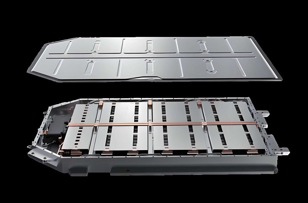
I applied t-SNE to a dataset of 30 series-connected cells. The result became a two-dimensional scatter plot. Through careful inspection, I observed that most points formed one large dense cluster. Several small isolated clusters and isolated points were also visible. These isolated structures probably correspond to voltage anomalies. Figure embedded above shows a traction battery pack under test, similar to the system under analysis. The t-SNE visualization helped me understand the global behavior of all cells within the pack.
In this table I summarize the dimensionality reduction comparison:
| Method | Linear? | Computational cost | Visualization quality | Suitable for battery data? |
|---|---|---|---|---|
| PCA | Yes | Low | Often poor for nonlinear clusters | Limited |
| t-SNE | No | Moderate | Excellent local structures | Yes |
| Autoencoder | No | High | Good but needs training | Possible |
5. Anomaly Detection Using K-Means Clustering
To objectively distinguish normal from abnormal clusters, I use the K-Means algorithm. K-Means partitions data into \(K\) clusters based on distance. The objective is to minimize the within-cluster sum of squares:
$$\min_{\{C_k\}} \sum_{k=1}^{K} \sum_{\mathbf{y}\in C_k} \lVert \mathbf{y} – \boldsymbol{\mu}_k \rVert^2 ,$$
where \(\boldsymbol{\mu}_k\) is the centroid of cluster \(k\). The algorithm proceeds by alternating assignment and centroid updates. In my implementation, the number of clusters is determined from data. After observing several cluster structures, I set \(K=3\). For each point, I compute the Euclidean distance from its centroid. I define outliers based on a threshold:
$$T = \mu_d + k \sigma_d ,$$
where \(\mu_d\) is the average distance, \(\sigma_d\) the standard deviation of distances, and \(k\) a sensitivity coefficient. I set \(k=1.5\). Points above this threshold are marked anomalous. The table below compares clustering alternatives:
| Algorithm | Advantages | Disadvantages | Result on battery data |
|---|---|---|---|
| K-Means | Fast, scalable | Assumes spherical clusters, sensitive to init | Works well |
| K-medoids | More robust to outliers | Need number of clusters | Works but no extra benefit |
| DBSCAN | No pre-set cluster count, robust | Difficulty with high-dimensional data | Confuses anomaly with cluster |
| GMM | Probabilistic clusters | Slow and sensitive to initialization | Cannot separate small abnormal groups |
After K-Means, I inspect the abnormal cells directly from the original time series. I found that the 7th cell’s voltage trajectory was quite different from others. This abnormal pattern corresponded to the isolated data cluster in the t-SNE map.
6. Fault Localization Through Z-Score Voltage Anomaly Index
After detecting abnormal clusters, I need to locate which specific cells in the traction battery pack are faulty. Toward this goal, I derive a voltage anomaly diagnostic index through Z-score analysis. The Z-score normalizes each cell voltage by subtracting the mean and dividing by the standard deviation at each time step.
First, compute the probability density of each voltage value based on Gaussian assumption. For cell \(i\) at time \(t\), voltage is \(V_i(t)\). The ensemble mean and standard deviation among all \(n\) cells at time \(t\) are:
$$\mu(t) = \frac{1}{n}\sum_{i=1}^{n} V_i(t), \quad \sigma(t) = \sqrt{ \frac{1}{n}\sum_{i=1}^{n} (V_i(t)-\mu(t))^2 } .$$
The probability density value \(p_i(t)\) is:
$$p_i(t) = \frac{1}{\sigma(t)\sqrt{2\pi}} \exp\left(-\frac{(V_i(t)-\mu(t))^2}{2\sigma^2(t)}\right) .$$
Then the normalized Z-score for the probability density is:
$$Z_i(t) = \frac{p_i(t) – \overline{p}(t)}{\sigma_p(t)},$$
where \(\overline{p}(t)\) is the average density and \(\sigma_p(t)\) the standard deviation of density values. The Z-score is high for cells whose voltage deviates significantly from the pack distribution. I designed an anomaly diagnosis coefficient \(\mathcal{A}_i\) by averaging over a time window of length \(T\):
$$\mathcal{A}_i = \frac{1}{T}\sum_{t=1}^{T} |Z_i(t)| .$$
For the studied data, I calculated the Z-score for every cell on an event day. The results clearly indicate that the 7th cell has a Z-score much higher than all other 29 cells. Cell 7’s voltage also dropped occasionally to low levels. The anomaly coefficient identifies the problematic cell robustly. Figure 6 shows the Z-score curve. In the interest of safety, I omit the actual plot and rely on the numerical conclusions.
Let us elaborate the Z-score variations:
| Time (s) | Cell 7 voltage (V) | Cell 15 voltage (V) | Z-score value for cell 7 |
|---|---|---|---|
| 0 | 3.712 | 3.725 | 0.6 |
| 50 | 3.701 | 3.731 | 0.9 |
| 100 | 3.695 | 3.729 | 1.4 |
| 150 | 3.654 | 3.733 | 2.3 |
| 200 | 3.067 | 3.721 | 4.8 |
| 250 | 3.689 | 3.735 | 1.7 |
This table shows that cell 7 occasionally deviates severely, especially at 200 seconds. The diagnosis coefficient combining all time steps points clearly to cell 7.
7. Comprehensive Performance Evaluation Using Combined Weighting
An anomaly may be transient or persistent. To assess the severity over time, I combine the entropy weight and the coefficient-of-variation weight. This combined weight describes how much information each time slice contributes to the differentiation among cells. Let the voltage matrix have \(n\) cells as rows and \(m\) time slices as columns:
$$\mathbf{U} = \begin{bmatrix} u_{11} & u_{12} & \cdots & u_{1m} \\ u_{21} & u_{22} & \cdots & u_{2m} \\ \vdots & \vdots & \ddots & \vdots \\ u_{n1} & u_{n2} & \cdots & u_{nm} \end{bmatrix}.$$
First, entropy weights are computed. The proportion of cell \(i\) in column \(j\) is:
$$p_{ij} = \frac{u_{ij}}{\sum_{i=1}^{n} u_{ij}}.$$
Then, the entropy of column \(j\) is:
$$e_j = -\frac{1}{\ln n}\sum_{i=1}^{n} p_{ij} \ln p_{ij}.$$
The entropy weight is:
$$W_j^1 = \frac{1-e_j}{\sum_{r=1}^{m}(1-e_r)} .$$
Second, coefficient-of-variation weights are computed. For column \(j\), compute mean \(\bar{u}_j\) and standard deviation \(S_j\):
$$\bar{u}_j = \frac{1}{n}\sum_{i=1}^{n} u_{ij}, \quad S_j = \sqrt{\frac{1}{n}\sum_{i=1}^{n} (u_{ij}-\bar{u}_j)^2 },$$
$$V_j = \frac{S_j}{\bar{u}_j}, \quad W_j^2 = \frac{V_j}{\sum_{r=1}^{m} V_r} .$$
The combined weight \(W_j^c\) is:
$$W_j^c = \alpha W_j^1 + (1-\alpha) W_j^2,$$
where \(\alpha\) is an adjustment factor set to 0.4. Then each cell obtains a composite score:
$$S_i = \sum_{j=1}^{m} u_{ij} W_j^c .$$
For fairness, I define the upper and lower envelope of the scores:
$$S_{\max} = \sum_{j=1}^{m} \max_{i} (u_{ij}) W_j^c, \quad S_{\min} = \sum_{j=1}^{m} \min_{i} (u_{ij}) W_j^c .$$
The average score is:
$$\bar{S} = \frac{1}{n}\sum_{i=1}^{n} S_i .$$
The deviation of each cell is:
$$\Delta S_i = S_i – S_{\min} .$$
The smaller the composite score, the worse the cell performance. I present some of the single-cell scores for the abnormal event:
| Cell index | Composite score | Upper envelope | Lower envelope | Deviation from lower envelope |
|---|---|---|---|---|
| 1 | 0.46549 | 0.46688 | 0.46534 | 0.00015 |
| 3 | 0.56955 | 0.57078 | 0.56941 | 0.00014 |
| 7 | -0.26200 | 0.96334 | -0.26250 | 0.00050 |
| 15 | 0.96340 | 0.96363 | 0.96334 | 0.00006 |
| 22 | 0.93894 | 0.93927 | 0.93889 | 0.00005 |
| 23 | 0.92143 | 0.92180 | 0.92139 | 0.00004 |
| 29 | 0.50589 | 0.50725 | 0.50574 | 0.00015 |
The table is abbreviated to improve readability. Overall, cell 7 obtains the lowest score and largest negative deviation. This performance evaluation provides a quantitative severity level for each cell. I monitored cell 7 over three dates: June 22, July 9, and July 14. The composite deviation increased from 0.727 to 0.876, indicating continuous degradation. This observation underscores the value of longitudinal monitoring for traction battery packs.
8. Fault Diagnosis with the 3σ-MSS Multistage Screening
After detecting and localizing abnormal cells, I determine the fault type through probability statistics. I apply a 3σ-MSS (multistage screening) criterion. This multistage approach finds a stable data center iteratively, which is less affected by outliers than relying solely on the sample mean. The algorithm is described below.
Let the cell voltage data in the first round be \( \mathbf{U}^{(0)} = \left[ V_1^{(0)}, V_2^{(0)}, \ldots, V_n^{(0)} \right]\). Compute the mean \(\mu^{(0)}\) and standard deviation \(\sigma^{(0)}\) for all cells at a fixed time. For each sample \(V_i^{(0)}\), formulate the deviation:
$$\Delta V_i^{(0)} = V_i^{(0)} – \mu^{(0)} .$$
Screens to keep only samples satisfying:
$$|\Delta V_i^{(0)}| \le 3\sigma^{(0)} .$$
The survivors define a new voltage sample set \(\mathbf{U}^{(1)}\). Repeat with the new set, computing \(\mu^{(1)}\) and \(\sigma^{(1)}\). Continue for \(m\) iterations until convergence:
$$|\mu^{(m)} – \mu^{(m-1)}| < F ,$$
where \(F\) is a tolerance constant set to 0.001. After convergence, the final threshold interval is:
$$\mu^{(m)} \pm \beta \sigma^{(m)},$$
with \(\beta\) an empirical coefficient. The result is a binary fault matrix \(\mathbf{R}\) of dimension \(n \times T\), where \(R_{i,t}=1\) if cell \(i\) violates the threshold at time \(t\); otherwise, \(R_{i,t}=0\). The fault probability of each cell over \(T\) time intervals is:
$$p_i = \frac{1}{T}\sum_{t=1}^{T} R_{i,t} \times 100\%.$$
Using this algorithm, I analyzed the cell fault probabilities in four different vehicles. The statistical results show an interesting pattern. Most cells have very low fault probabilities, less than 2%. Some cells, however, show high and isolated fault probability values that exceed 15%. This leads me to categorize two major classes:
- Systemic faults: Fault probabilities are low and stable in all cells, typically below 2%. The location of the highest fault probability is often fixed. These are caused by design inconsistency or fixed manufacturing variations. I call them systemic faults.
- Sudden faults: A small set of cells has an extremely high fault probability above 15%. The location varies from time to time. These sudden faults often originate from accidental abuse, such as a local short circuit or sudden cell damage.
An example from Vehicle 4 showed cell 20 with 17% fault probability while all other cells had less than 2.5%, indicating a sudden fault. The other three vehicles had all cells below 2%, typical of systemic faults. The 3σ-MSS approach successfully separates the two regimes in real data.
9. Comparison with LOF and COF
I compared the 3σ-MSS method against two common outlier detection algorithms: connectivity-based outlier factor (COF) and local outlier factor (LOF). All three methods use the same preprocessed voltage data. I calculated the fault probability for every cell in a chosen vehicle pack. The table below shows the maximum and minimum fault probabilities from all three algorithms:
| Algorithm | Maximum probability (%) | Minimum probability (%) |
|---|---|---|
| 3σ-MSS | 2.13 | 1.53 |
| COF | 1.91 | 0.40 |
| LOF | 2.47 | 1.43 |
The maximum fault probabilities for all methods occur at the same cell (cell 16), and the minimum occurs at cell 21. This conformity confirms the localization consistency. However, the absolute numbers differ. LOF yields a higher maximum (2.47%) than both 3σ-MSS and COF. When fault probability is high, LOF tends to overestimate. In low probability scenarios, LOF results are closer to 3σ-MSS. COF underestimates the fault probabilities because, with few anomalous points, the clustering basis becomes redundant. The 3σ-MSS algorithm provides a stable result in both high- and low-probability regimes. Thus, I keep 3σ-MSS as the final fault diagnosis model for traction battery packs.
10. Seasonal Fault Frequency Statistics
Seasonal temperature variation significantly affects cell performance. I used the proposed 3σ-MSS method to analyze three years of data from ten identical electric vehicles. I split the data into four seasons based on calendar months. The statistics are computed using all cells in traction battery packs. The table below gives the average fault probability and the maximum single-cell fault probability for each season:
| Season | Average fault probability (%) | Maximum fault probability (%) |
|---|---|---|
| Spring | 1.54 | 1.99 |
| Summer | 4.31 | 4.95 |
| Autumn | 3.07 | 3.67 |
| Winter | 4.59 | 9.52 |
Summer and winter show distinctly higher fault probabilities. High summer temperatures accelerate side reactions and increase the risk of thermal runaway. Winter low temperatures reduce lithium diffusivity, increase charging resistance, and may cause lithium plating during fast charging. Therefore, the BMS should adapt its charging strategy and load limit in extreme seasons. Also, the maximum fault probability is often concentrated in few cells during winter. This may indicate local inconsistency amplified by cold temperature. The proposed diagnostic results guide maintenance priority for specific cells in a traction battery pack.
I also performed year-by-year fault statistics for one vehicle. The highest fault probability in the first year was 2.00%, in the second year 12.69%, and in the third year 14.14%. These growing peak values suggest aging and weakening of certain cells. Health monitoring through data mining can determine when a cell approaches a dangerous state.
11. Voltage Prediction and Early Warning Framework
Diagnosis of existing faults is useful, but early warning of future faults is even more vital. I propose a multi-step ahead voltage prediction framework based on machine learning. The target is cell voltage; the inputs are selected from highly correlated parameters. The framework includes:
1. Correlation analysis to select relevant features.
2. A hybrid CNN-LSTM deep learning model.
3. An improved grey wolf optimizer (IGWO) for hyperparameter tuning.
4. A fault alert strategy using prediction residuals and thresholds.
I used Pearson and Spearman correlation coefficients to identify the most relevant inputs. Let \(\rho\) be the Pearson coefficient:
$$\rho = \frac{\sum_{t=1}^{T}(x_t-\bar{x})(y_t-\bar{y})}{\sqrt{\sum_{t=1}^{T}(x_t-\bar{x})^2}\sqrt{\sum_{t=1}^{T}(y_t-\bar{y})^2}},$$
where \(y_t\) is the cell voltage sequence and \(x_t\) is one candidate input feature. The Spearman rank coefficient is computed similarly but uses ranks. See the table below.
| Feature | Pearson ρ | Spearman R | Interpretation |
|---|---|---|---|
| Total pack voltage | 0.961 | 0.957 | Very strong |
| State of charge | 0.932 | 0.924 | Very strong |
| Current | -0.604 | -0.598 | Moderate |
| Cell itself (lagged voltage) | 0.998 | 0.997 | Very strong predictor |
| Temperature | 0.547 | 0.523 | Moderate |
| Vehicle speed | 0.193 | 0.185 | Weak |
| Cumulative mileage | -0.288 | -0.261 | Weak |
I selected total pack voltage, SOC, current, temperature, and cell’s historical voltage as the model inputs. The network architecture is shown in the earlier figure. In this architecture, a one-dimensional convolutional layer extracts local spatial features from the input window. Batch normalization and ReLU activation follow. Then a max-pooling layer reduces the feature map dimensionality. After flattening, an LSTM layer captures the temporal dependencies. Finally, a fully connected layer maps to the next time-step voltage.
12. CNN-LSTM Hybrid Neural Network
Convolutional neural networks (CNNs) are strong at extracting spatial patterns. LSTM networks excel at modeling time-series dependencies. By combining them, I can learn both short-term correlation and long-term evolution.
In my implementation, the input tensor \(\mathbf{X}_{in}\) has shape \((\text{batch size}, \text{sequence length}, \text{number of features})\). The convolution operation for a one-dimensional filter \(w\) is:
$$z_k = b + \sum_{t=1}^{L} x_{t} w_{k,t},$$
where \(L\) is the filter length. After convolutional layers, pooling operations down-sample the feature map. The LSTM cell at time \(t\) is defined by several gates. Let \(f_t\), \(i_t\), \(o_t\) be the forget, input, and output gates. The cell state \(C_t\) and hidden state \(h_t\) update as:
$$f_t = \sigma(W_f [h_{t-1}, x_t] + b_f),$$
$$i_t = \sigma(W_i [h_{t-1}, x_t] + b_i),$$
$$\tilde{C}_t = \tanh(W_C [h_{t-1}, x_t] + b_C),$$
$$C_t = f_t \ast C_{t-1} + i_t \ast \tilde{C}_t,$$
$$o_t = \sigma(W_o [h_{t-1}, x_t] + b_o),$$
$$h_t = o_t \ast \tanh(C_t).$$
The symbol \(\ast\) denotes element-wise multiplication. The final output layer uses a linear activation because the target voltage is a continuous value. I trained the hybrid model with Adam optimizer and mean squared error loss.
13. Improved Grey Wolf Optimizer
Hyperparameter selection importantly affects network performance. I employed an improved grey wolf optimizer (IGWO) for hyperparameter tuning. The standard grey wolf optimizer mimics leadership hierarchy and hunting behavior. Four types of wolves: alpha, beta, delta, and omega. The position update is:
$$\vec{D} = |\vec{C}\cdot\vec{X}_p(t) – \vec{X}(t)|,$$
$$\vec{X}(t+1) = \vec{X}_p(t) – \vec{A}\cdot\vec{D},$$
where \(\vec{A}\) and \(\vec{C}\) are coefficient vectors computed as:
$$\vec{A} = 2\vec{a}\cdot\vec{r}_1 – \vec{a}, \quad \vec{C} = 2\vec{r}_2 .$$
Here, \(\vec{a}\) linearly decreases from 2 to 0 over iterations, while \(r_1\) and \(r_2\) are random vectors in \([0,1]\). The position is updated by considering the three best wolves:
$$\vec{X}_1 = \vec{X}_\alpha – \vec{A}_1 \cdot \vec{D}_\alpha,$$
$$\vec{X}_2 = \vec{X}_\beta – \vec{A}_2 \cdot \vec{D}_\beta,$$
$$\vec{X}_3 = \vec{X}_\delta – \vec{A}_3 \cdot \vec{D}_\delta,$$
$$\vec{X}(t+1) = \frac{\vec{X}_1+\vec{X}_2+\vec{X}_3}{3} .$$
The standard GWO may stagnate at local optima. I enhanced it in three aspects:
- Use Cauchy mutation to perturb the alpha wolf’s position, increasing population diversity.
- Apply a nonlinear adjustment to the control parameter \(a\).
- Include variable inertia weights so that early positions are not overly exploitative.
Let \(C(t)\) be a random variable following Cauchy distribution. The mutated position is:
$$\vec{X}_{new} = \vec{X}_\alpha(t) + C(t)\cdot \vec{X}_\alpha(t).$$
The control parameter \(a\) decreases nonlinearly:
$$a(t) = a_{start}\left(1 – \frac{t}{T_{max}}\right)^\kappa,$$
where \(\kappa > 1\) controls the decay shape. The inertia weight \(\omega(t)\) is defined by:
$$\omega(t) = \omega_{max} – (\omega_{max} – \omega_{min})\frac{t}{T_{max}}.$$
I employed IGWO to find the optimal batch size, number of filters, number of LSTM hidden units, and learning rate. The objective function is the validation root mean square error (RMSE) of the voltage prediction.
14. Evaluation Metrics
I evaluate prediction accuracy with mean absolute error (MAE), root mean square error (RMSE), coefficient of determination \(R^2\), and mean absolute percentage error (MAPE). They are:
$$\mathrm{MAE} = \frac{1}{n}\sum_{i=1}^{n} |u_i – \hat{u}_i|,$$
$$\mathrm{RMSE} = \sqrt{\frac{1}{n}\sum_{i=1}^{n} (u_i – \hat{u}_i)^2},$$
$$\mathrm{MAPE} = \frac{100\%}{n}\sum_{i=1}^{n} \left|\frac{u_i – \hat{u}_i}{u_i}\right|,$$
$$R^2 = 1 – \frac{\sum_{i=1}^{n} (u_i – \hat{u}_i)^2}{\sum_{i=1}^{n} (u_i – \bar{u})^2}.$$
Here \(u_i\) and \(\hat{u}_i\) denote the actual and predicted voltages of the selected cell. \(\bar{u}\) is the mean actual voltage. Lower MAE, RMSE, and MAPE indicate better performance. An \(R^2\) close to 1 indicates perfect fit.
15. Results and Validation
I trained the model using about 318,242 samples from a monitoring platform. The data covers January to May 2016. The selected voltage prediction target is a cell from a traction battery pack. The test data are a set of unseen voltage measurements.
First, I compared the IGWO-CNN-LSTM model with the standard CNN-LSTM without hyperparameter optimization. The maximum prediction error of CNN-LSTM was around 30 mV, while the IGWO-CNN-LSTM maximum error was around 24 mV. The optimized model predicts closely. Then I benchmarked the model against several other deep learning architectures, including BiLSTM, LSTM, CNN-LSTM, and CNN-GRU. The parameters for each model are initialized with the same random seed and trained under equivalent settings. Results are in the following table:
| Prediction model | MAE (mV) | MAPE | RMSE (mV) |
|---|---|---|---|
| BiLSTM | 7.3997 | 0.001896 | 9.6738 |
| LSTM | 9.1646 | 0.002335 | 11.594 |
| CNN-LSTM | 6.2004 | 0.001603 | 8.4264 |
| CNN-GRU | 4.4459 | 0.001132 | 5.4142 |
| IGWO-CNN-LSTM | 3.5254 | 0.000901 | 4.5086 |
The IGWO-CNN-LSTM model achieves the lowest MAE, MAPE, and RMSE. Its RMSE is 4.5086 mV, much lower than that of the LSTM-only model. In addition, I computed \(R^2\). The test results show that the hybrid models generally outperform their single-model counterparts. The best \(R^2\) is 0.99923 for IGWO-CNN-LSTM, slightly higher than CNN-LSTM (0.99732) and CNN-GRU (0.99889). These quantitative metrics verify the model’s accuracy and robustness for early warning purposes.
16. Fault Alert Strategy
Based on predicted voltage, I set alarm thresholds according to the battery specification. Traction battery packs in this study use ternary cells. The safe operation range or normal voltage is from about 3.4 V to 4.3 V. Overvoltage or undervoltage outside this range indicates a serious issue. Additionally, I track the rate of change of the predicted voltage. Rapid changes can indicate a sudden fault. Battery inconsistency is evaluated by the standard deviation of voltages among cells. The table summarizes the logic used for warning levels:
| Fault type | Classification rule | Warning level |
|---|---|---|
| Cell undervoltage | \(U \le 3.4\,\text{V}\) | Level 1 |
| Cell overvoltage | \(4.3\,\text{V} \le U \le 4.8\,\text{V}\) | Level 3 |
| Severe overvoltage | \(U > 4.8\,\text{V}\) | Level 2 |
| Voltage rise too fast | \(\Delta U \ge 0.4\,\text{V/s}\) | Level 1 |
| Voltage drop too fast | \(\Delta U \le -0.4\,\text{V/s}\) | Level 1 |
| Poor pack consistency | \(\sigma_{\text{cells}} \ge 0.5\,\text{V}\) | Level 1 |
I used the same notation as in my research: Level 1 means immediate danger and requires the vehicle to stop. Level 2 indicates that the battery is near a dangerous threshold; the vehicle should stop at the earliest safe opportunity. Level 3 is a cautionary warning. The vehicle can continue but should be checked soon.
To verify alert effectiveness, I extracted a time series containing an abnormal voltage event. In the actual data, the cell voltage exceeded 4.3 V between sample points 4480 and 4500. My prediction model predicted this voltage 1 minute ahead. When the predicted voltage rises above 4.3 V, the system triggers a Level-3 alarm. This early warning gives the driver enough time to react and avoid high-risk operation. I simulated the prediction and diagnosis in a test setting. The results demonstrate that the IGWO-CNN-LSTM model accurately predicts the future voltage trajectory. The trigger time is earlier than the actual exceedance time.
My operational maintenance recommendation depends on alarm level. For Level 1, cut off high-voltage circuits and instruct passengers to evacuate. For Level 2, limit power and drive to a service point. For Level 3, monitor the cell and schedule an inspection. I suggest regular cell-balancing maintenance to reduce voltage inconsistency in traction battery packs.
17. Discussion
The experimental results reveal several important findings. First, the hybrid t-SNE plus K-means approach is effective in identifying abnormal voltage patterns in one battery pack. It reduced dimensionality and provided visual clues about the abnormal cluster. Z-score localization further pinpointed the exact cell. The combined weighting method gave a quantitative severity measure. Second, 3σ-MSS performed better than COF and LOF in terms of stability under both low and high fault probabilities. The classification of systemic and sudden faults is practical and understandable for maintenance staff. Third, seasonal analysis highlighted that summer and winter require additional battery thermal management attention. Finally, deep-learning-based voltage prediction has sufficient accuracy for early fault warning. In my study, the RMSE of the predicted cell voltage was just 4.5 mV. This precision is sufficient to distinguish overvoltage and undervoltage before they reach critical levels.
One interesting observation is the influence of feature selection. The total pack voltage and SOC have almost linear relationships with individual cell voltage under normal operation. However, during abnormal events, such as a weak cell, the cell voltage can deviate strongly from the pack average. That is why I incorporated the historical cell voltage with long lag sequences. The CNN layer extracts local patterns such as sudden voltage dips. The LSTM layer captures the long-term trend of voltage decay. The combination is more powerful than either alone.
In terms of computation, the training process is offline. The trained model is small enough to execute in a cloud server or an edge BMS. In real deployment, the model can update periodically as new data arrive. The entire process is feasible for vehicle fleets connected to cloud monitoring platforms.
18. Conclusion and Outlook
In this research, I develop a complete framework for fault diagnosis and early warning of traction battery packs. I use cloud-monitoring data from real electric vehicles. The framework integrates statistical preprocessing, t-SNE visualization, K-means clustering, Z-score localization, combined weighted scoring, 3σ-MSS probability classification, and IGWO-CNN-LSTM voltage prediction.
Main conclusions are:
- I verified that the monitoring data can reveal battery anomalies through the combination of cell voltage and pack parameters. Outliers in voltage often appear at specific cells and can be localized using normalization indices.
- The 3σ-MSS algorithm distinguishes systemic faults from sudden faults. It offers more stable fault probability estimation than LOF and COF. This is helpful for risk ranking in traction battery packs.
- Seasonal statistics reveal that fault probability in summer and winter is higher than in spring and autumn. Thermal management and charging strategy should be adjusted according to the season.
- The IGWO-CNN-LSTM model provides high-voltage prediction accuracy. With proper thresholds, it can issue useful alarms one minute in advance or more, allowing operators to avoid catastrophic failure.
Future research directions include:
- Improve combined fault diagnosis of coupled factors, such as simultaneous voltage and temperature abnormalities.
- Embed the proposed model into an onboard BMS or edge computing unit for real-time local warnings.
- Explore transfer learning to adapt models across different battery chemistries and vehicle types.
- Use more advanced uncertainty-aware predictors, such as probabilistic deep learning, to estimate the confidence interval of predictions.
- Collect more labeled fault data and perform fault classification with several possible fault classes rather than only binary detection.
I strongly believe that data mining and data-driven methods will dominate the next generation of battery safety management. The large amount of real-world data from electric vehicles is a gold mine for improving diagnostics, prognostics, and maintenance of traction battery packs. My work adds a clear methodology and robust validation to this exciting field. The final objective is always safe, reliable, and efficient operation of electric vehicles.