
1. Introduction
With the rapid development of the global automotive industry, the dependence on fossil fuels has brought increasingly severe challenges of energy shortage and environmental pollution. Traditional internal combustion engine vehicles emit a large amount of carbon dioxide and harmful pollutants, which are regarded as major contributors to global climate change and urban air quality deterioration. In this context, the pure electric vehicle, with its advantages of zero tailpipe emission, high energy conversion efficiency and low operating noise, has become one of the most important technology routes for the transformation of the automotive industry. For many countries, large-scale deployment of electric vehicles has been placed at the core of their national energy strategy, because it offers a practical pathway toward low-carbon transportation and sustainable mobility.
Over the past decade, the electric vehicle market has expanded remarkably. In the period between 2016 and 2018, market growth was mainly driven by purchase subsidies and policy incentives. After a short fluctuation caused by subsidy phase-out and external uncertainties around 2019, the market entered a rapid growth stage after 2021, with annual production and sales growing explosively. By 2025, annual production and sales of new energy vehicles in China surpassed sixteen million units, which indicates that the industry has entered a stage of market-oriented and mature development, with pure electric vehicles remaining the dominant product category. This growth trend is accompanied by increasing expectations from customers regarding driving range, safety, ride comfort and cost-effectiveness, which places higher demands on the development of core electronic control systems, especially the vehicle control unit (VCU).
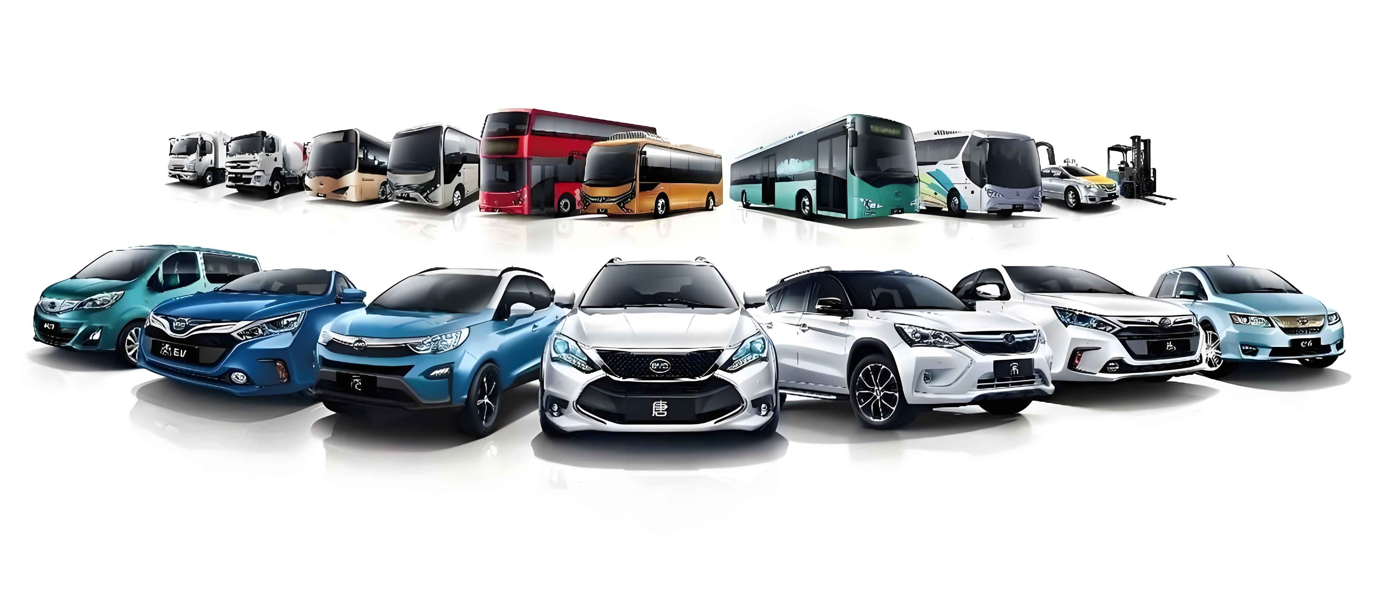
In the electric vehicle architecture, the VCU acts as the central decision-making unit. It acquires driver inputs from the accelerator pedal, brake pedal, gear selector and various vehicle states, coordinates the battery management system (BMS) and the motor control unit (MCU), and finally outputs torque requests and power management commands. For this reason, the control strategies embedded in the VCU directly determine the power performance, driving economy, safety and ride comfort of the whole vehicle. Among all functionalities, longitudinal control is the most fundamental part because it manages acceleration, deceleration, speed holding and energy recuperation. Nevertheless, conventional longitudinal control strategies often rely on fixed-parameter controllers, such as PID controllers or static look-up tables. In complex real-world driving conditions, these methods may not be robust enough, leading to insufficient parameter adaptivity in cruise control and non-optimal trade-offs between braking safety and regenerative efficiency.
Therefore, this study focuses on longitudinal control strategies of a pure electric vehicle. Taking a front-wheel-drive passenger car as the research platform, the work covers powertrain parameter matching and plant modeling, design of the basic VCU control logic, model-based optimization of the cruise control and regenerative braking strategies, and finally a comprehensive hardware-in-the-loop (HIL) test validation. By carrying out systematic closed-loop development from the virtual environment to the physical controller, the study aims to improve the cruise smoothness and energy efficiency of electric vehicles in practical operation.
2. Powertrain Parameter Matching and Vehicle Plant Modeling
2.1 Vehicle architecture and key design indicators
The target vehicle in this work adopts a front-wheel-drive layout. The powertrain system consists of a permanent magnet synchronous motor (PMSM), a fixed-ratio single-speed reducer, an inverter, and a lithium-ion battery pack. The electric machine is mechanically connected to the differential through the reducer with a gear ratio of 6.8. A simplified but representative configuration of power flow is as follows: during normal driving, electrical energy is drawn from the battery and converted into mechanical torque by the motor; during deceleration or braking, the motor operates in generating mode and the recovered energy is stored back into the battery. The high-level signal flow between the driver, the VCU, the motor controller and the battery management system realizes the coordinated control of the vehicle.
Before the control layer is developed, the key vehicle parameters must be defined because the vehicle controller and the virtual plant used in the simulation should share the same physical constraints. The most important vehicle parameters used in this study are summarized in the following table.
| Parameter | Symbol | Value |
|---|---|---|
| Curb mass | \( m_c \) | 1285 kg |
| Gross mass | \( m_a \) | 1715 kg |
| Air drag coefficient | \( C_D \) | 0.31 |
| Rolling resistance coefficient | \( f \) | 0.014 |
| Tire rolling radius | \( r \) | 305 mm |
| Frontal area | \( A \) | 1.96 m² |
| Rotational mass conversion factor | \( \delta \) | 1.08 |
| Wheelbase | \( L \) | 2720 mm |
| Final drive ratio | \( i_0 \) | 6.8 |
| Drivetrain efficiency | \( \eta_t \) | 0.97 |
The objective performance requirements of the vehicle are a maximum speed of at least 140 km/h, a maximum gradeability above 25%, an acceleration time from 0 to 100 km/h no greater than 12 seconds, an acceleration time from 30 to 90 km/h no greater than 8 seconds, and a driving range of more than 300 km under constant-speed conditions. These indicators serve as the design constraints for the electric machine and battery sizing.
2.2 Drive motor parameter matching
The rated power and peak power of the traction motor have to be selected so that the motor can satisfy the power demand in three representative operating conditions: maximum speed, maximum grade, and acceleration. For the maximum-speed condition, the vehicle is considered to run on a flat road at the maximum speed \(v_{\max}=150\) km/h. The required motor power is obtained from the longitudinal driving equation:
$$ P_{v\max} = \frac{1}{\eta_t} \left( \frac{m g f v_{\max}}{3600} + \frac{C_D A v_{\max}^3}{76140} \right) \approx 39.5\ \text{kW}. $$
This result gives the lower boundary for the sustained power output of the motor.
For the grade-climbing condition, the vehicle is assumed to climb a 20% grade at 30 km/h. The required power is:
$$ P_{\text{slope}} = \frac{1}{\eta_t} \left( \frac{m g f \cos\alpha \, v_s}{3600} + \frac{m g \sin\alpha\, v_s}{3600} + \frac{C_D A v_s^3}{76140} \right) \approx 36.2\ \text{kW}, $$
where \(\alpha=\arctan(0.2)\) is the slope angle. In this condition, a relatively large torque at low speed is necessary, which is covered by the peak torque capability of the motor.
For the acceleration condition, the vehicle accelerates from standstill to 100 km/h within \(t_{acc}=12\) s. A simplified average power demand can be expressed as:
$$ P_{acc} \approx \frac{1}{\eta_t} \left( \frac{\delta m v_{acc}^2}{2 t_{acc}} + \frac{m g f v_{acc}}{3600} + \frac{C_D A v_{acc}^3}{76140} \right) \approx 95\ \text{kW}. $$
In the above expression, the first term accounts for the kinetic energy increase of both translational and rotational masses, while the remaining terms cover rolling and aerodynamic losses. Considering a certain power margin and the thermal endurance in high-power operations, a motor with a peak power of 100 kW and a rated power of 45 kW is selected.
The maximum torque is determined from the gradeability requirement. For a vehicle climbing a 20% grade at low speed, the required tractive torque at the motor shaft is:
$$ T_{\max} \ge \frac{r (m g f \cos\alpha + m g \sin\alpha)}{i_0\, \eta_t} \approx 245\ \text{N·m}. $$
Consequently, the selected motor provides a maximum torque of 320 N·m, which gives additional torque reserve for transient driving conditions. The maximum motor speed must cover the vehicle speed of 150 km/h. Using the rolling radius and the final drive ratio:
$$ n_{\max} = \frac{v_{\max} i_0}{0.377\, r} \approx 9018\ \text{r/min}. $$
Therefore, the maximum motor speed is finally chosen as 10000 r/min. The basic specifications of the traction motor are listed below.
| Parameter | Value |
|---|---|
| Motor type | Permanent magnet synchronous motor |
| Rated power | 45 kW |
| Peak power | 100 kW |
| Peak torque | 320 N·m |
| Rated speed | 3000 r/min |
| Maximum speed | 10000 r/min |
2.3 Power battery parameter matching
The battery capacity is selected according to the required driving range. For the target range of 400 km at a constant speed of 60 km/h, the total required battery energy can be estimated as:
$$ W_m = P_{60} \cdot \frac{S}{v_{60}} \approx 51.2\ \text{kWh}, $$
where \(P_{60}\) is the power demand at 60 km/h. A lithium-ion battery pack with a nominal voltage of 320 V and a capacity of 160 Ah is selected. The total stored energy is then calculated as:
$$ W_b = \frac{U C}{1000} = \frac{320 \times 160}{1000} = 51.2\ \text{kWh}. $$
This configuration satisfies the long-distance driving objective while leaving appropriate margins for auxiliary loads, battery aging and regenerative charging. The key battery parameters are summarized below.
| Parameter | Value |
|---|---|
| Battery type | Lithium-ion |
| Rated voltage | 320 V |
| Rated capacity | 160 Ah |
| Total energy | 51.2 kWh |
| Usable SOC window | 5%–100% |
2.4 Vehicle plant modeling in Simulink
To support the upstream development of the VCU software and the subsequent hardware-in-the-loop tests, a complete vehicle model is built in MATLAB/Simulink. This virtual plant includes the driver model, the electric machine model, the battery model and the longitudinal vehicle dynamics model.
2.4.1 Driver model
The driver model converts a reference speed trajectory into accelerator and brake pedal signals. It is implemented as a PI controller. The speed error is defined as:
$$ e(t)=v_{\text{ref}}(t)-v_{\text{act}}(t). $$
The control output is then generated according to the PI rule:
$$ u(t) = K_p e(t) + K_i \int_{0}^{t} e(\tau)\,d\tau. $$
When the controller output \(u(t)\) is positive, the signal is interpreted as an accelerator pedal command; when negative, its absolute value is taken as the brake pedal command. Both pedal signals are saturated in the interval \([0, 1]\), representing the physical limits of the two pedals. This driver model supplies the vehicle controller with realistic driver inputs.
2.4.2 Electric machine model
The motor model is built for energy-oriented simulation rather than for electromagnetic transient studies. Therefore, the electrical machine characteristics are represented by quasi-static maps. The input of the model is the target torque requested by the VCU, while the outputs include the actual torque delivered to the driveline, the electric power consumption and the battery-side current. The maximum torque at a given speed is obtained from the motor envelope curve. The theoretical output torque is given by:
$$ T_{\text{theo}} =
\begin{cases} T_{\max}, & T_{\text{ref}}>T_{\max} \\ T_{\text{ref}}, & -T_{\max}\le T_{\text{ref}}\le T_{\max} \\ -T_{\max}, & T_{\text{ref}}<-T_{\max} \end{cases}. $$
Then the electrical power request is calculated as
$$ P_{\text{req}} = \frac{T_{\text{theo}}\, n}{9550\, \eta} $$
in the driving mode, and as
$$ P_{\text{req}} = \frac{T_{\text{theo}}\, n\, \eta}{9550} $$
during regenerative braking. The requested power is further limited by the maximum permissible charging or discharging power of the battery. In this way, the model can emulate the coupling behavior of the motor and battery systems in a simple but effective manner.
2.4.3 Battery model
The battery is modeled using the ampere-hour integration method for SOC estimation, and a second-order RC equivalent-circuit network for voltage calculation. The terminal voltage of the battery can be expressed as:
$$ V_{t}=E(I_{\text{batt}},SOC)-I_{\text{batt}} R_0 – U_{RC1} – U_{RC2}. $$
Each RC network represents a polarization process, with the dynamic voltage determined by:
$$ \frac{dU_{RCi}}{dt} = \frac{I_{\text{batt}}}{C_i} – \frac{U_{RCi}}{R_i C_i}. $$
The SOC is calculated as:
$$ SOC(t)=SOC(0)-\frac{1}{C}\int_{0}^{t} \eta_{\text{coul}} I_{\text{batt}}(\tau)\,d\tau, $$
where \(\eta_{\text{coul}}\) denotes the coulombic efficiency. The battery model also imposes instantaneous charge and discharge current limits according to the predefined battery boundaries.
2.4.4 Longitudinal vehicle dynamics model
The longitudinal motion of the electric vehicle is governed by the equilibrium of the tractive force and the driving resistances. In the driving mode, the equation of motion reads:
$$ \frac{T_{tq} i_0 \eta_t}{r}=G f \cos\alpha+\frac{C_D A v^2}{21.15}+G\sin\alpha+\delta m \frac{dv}{dt}. $$
Therefore, the longitudinal acceleration can be solved as:
$$ \frac{dv}{dt}=\frac{1}{\delta m}\left(\frac{T_{tq} i_0 \eta_t}{r} – G f \cos\alpha – \frac{C_D A v^2}{21.15} – G\sin\alpha\right). $$
In the braking condition, the regenerative braking force \(F_{\text{reg}}\) and the hydraulic braking force \(F_{\text{mec}}\) are introduced into the balance equation together with the resistance forces, which forms the basis for the subsequent design and simulation of the regenerative braking controller:
$$ \frac{T_{\text{reg}}}{r}+F_{\text{mec}}+G f\cos\alpha + \frac{C_D A v^2}{21.15}+G\sin\alpha=-\delta m\frac{dv}{dt}. $$
2.5 Initial plant validation results
With the vehicle plant model completed, several simulation tests were run to verify whether the power matching satisfies the design indicators. In the maximum vehicle speed test, the simulated vehicle reaches 152.4 km/h and remains stable during a sustained high-speed cruise condition, proving that the powertrain can overcome the total resistance at highway speeds without thermal or torque boundary issues.
In the gradeability test, the simulated vehicle achieves 25.82% at standstill. Even at 80 km/h, the remaining gradeability is 9.54%, which is sufficient for normal highway and mountain applications.
The acceleration performance simulation shows that the vehicle accelerates from 0 to 100 km/h in 11.6 seconds, and from 30 to 90 km/h in 8.0 seconds. Both values are within the targets of 12 and 8 seconds, as summarized in the table.
| Performance indicator | Design objective | Simulation result |
|---|---|---|
| Maximum vehicle speed | ≥140 km/h | 152.4 km/h |
| Maximum gradeability | ≥25% | 25.82% |
| 0–100 km/h acceleration time | ≤12 s | 11.6 s |
| 30–90 km/h acceleration time | ≤8 s | 8.0 s |
| Driving range at 50 km/h | ≥300 km | 559.6 km |
| Driving range at 70 km/h | ≥300 km | 428.0 km |
The verified plant model is subsequently used as a virtual controlled plant in the development and testing of the VCU strategies, providing consistent longitudinal dynamic responses for the whole development chain.
3. Basic VCU Strategy Architecture
The basic control software of the VCU is organized in a modular architecture in Simulink/Stateflow. To maintain a clear boundary for the longitudinal control study, the software is divided into six major functional modules: input signal acquisition, power-up and power-down management, torque control system, cruise control, accessory control and fault diagnosis. The following table lists the modules and their main responsibilities.
| Module | Typical functions |
|---|---|
| Input signal parsing and conditioning | Analog/digital acquisition, plausibility check and filtering |
| Power management | Low-voltage wake-up, high-voltage Precharge timing |
| Torque control system | Torque map, creep control, power limitation, ramp filtering |
| Cruise control | Speed holding request and arbitration with driver torque |
| Accessory control | Cooling fan, water pump, lights and vacuum pump control |
| Fault diagnosis | Fault grading, limiting actions and error handling |
3.1 Input signal conditioning
The input module receives physical signals from the hardware interface, classifies them into hard-wired inputs and CAN inputs, and then passes the conditioned values to the control modules. Digital input signals are debounced using a Stateflow finite state machine. The debounce logic only updates the output logical state when the signal remains at the new level for a predefined number of processing cycles. This prevents chattering and spurious noise from causing erroneous switching in high-level logic.
Analog input signals, especially the two accelerator pedal position sensors, require careful conditioning. Two independent voltage signals \(V_1\) and \(V_2\) are monitored. During normal operation they should follow a prescribed proportionality. The plausibility check module verifies the ratio of the two voltages; if a short circuit or a broken wire drives the difference outside the safety window, the resulting pedal opening is forced to zero so that unintended acceleration is avoided. After this check, a rate-limit filter is used to suppress abrupt voltage jumps:
$$ V_{\text{out}}(k)=
\begin{cases}
V_{\text{in}}(k), & |V_{\text{in}}(k)-V_{\text{out}}(k-1)|\le \Delta V_{\max}\\
V_{\text{out}}(k-1), & |V_{\text{in}}(k)-V_{\text{out}}(k-1)|> \Delta V_{\max}
\end{cases}.
$$
Thereafter, a median filter is applied to remove high-frequency noise. Finally, each sensor voltage is converted to a pedal opening percentage:
$$ Acc_1=\frac{V_1-V_{1,\text{low}}}{V_{1,\text{high}}-V_{1,\text{low}}}\times 100\%. $$
The final accelerator pedal opening is the average of the two normalized sensor values. The simulation results in this research show that the raw signals contaminated with spikes are effectively smoothed, and the recovered pedal output is stable enough for torque request generation.
3.2 Power-up and power-down management
The high-voltage electrical system comprises a battery pack, an inverter with large DC-link capacitors and several high-voltage contactors. Because the initial voltage across the DC-link capacitors is zero, directly closing the main positive contactor could create a dangerous inrush current. Therefore, a precharge circuit is installed in parallel with the main positive contactor. During the precharge phase, the precharge contactor is closed first, and the current is limited by the precharge resistor. The main contactor is closed only after the bus voltage reaches a sufficiently high fraction of the battery voltage, for example 90% or above; then the precharge contactor is opened.
The low-voltage power-up logic is implemented as a state machine with the states INIT, SELF_CHECK, STANDBY and SELF_CHECK_FAILED. After the key-on signal wakes the controller, the VCU performs self-checks on the BMS, MCU and other critical ECUs. If all feedback messages are normal, the state machine enters STANDBY and evaluates the high-voltage enabling conditions.
The high-voltage power-up sequence is also implemented as a state machine. The main flow is described below.
| Step | Action | Exit condition |
|---|---|---|
| 1 | VCU sends power-on request to BMS | BMS closes main negative and precharge contactors |
| 2 | VCU waits for precharge finish | Bus voltage difference lower than 15 V |
| 3 | Main positive contactor is closed | Positive relay feedback is received |
| 4 | DCDC converter is enabled | DCDC output reaches target voltage |
| 5 | Motor inverter is enabled | MCU reports ready status |
| 6 | VCU enters READY state | Vehicle is ready for driving |
During every stage, the VCU monitors the feedback signals and includes a timeout protection. If the expected feedback is not received within a calibrated time, the entire power-up procedure is aborted and the system switches to the corresponding fault state. In the power-down path, the VCU first removes the driving enable and DCDC enable commands, then requests the BMS to disconnect the main relays. After the main relays are opened, the inverter performs an active discharge of the bus voltage below 60 V. If the main-relay opening process times out, an active discharge is skipped to avoid overloading the discharge resistor.
3.3 Torque control module
The torque control module calculates the total driveline torque request according to powertrain status, driver inputs and safety constraints. It is the most important part of the longitudinal control framework. The first submodule handles gear position management. To avoid unintentional and dangerous gear shifting, the shift demand is accepted only when the corresponding enable conditions are satisfied. For example, shifting from Park or Neutral into Drive requires a ready state, a pressed brake pedal, a valid Drive command and a vehicle speed below a predefined threshold. Similar logic is implemented for Reverse. This gear management state machine prevents transmission or motor damage during high-speed gear changes.
After the active gear is confirmed, the drive torque calculation module determines whether creep control or driver acceleration is requested. The core torque map takes the accelerator pedal opening and the motor speed as inputs, while the driving mode index distinguishes the economy mode from the normal mode. In addition, the drive torque is disabled if the brake pedal is pressed. In the energy-recovery branch, the torque control module monitors the brake pedal signal and motor speed. A one-dimensional map gives the base regenerative torque, which is then multiplied by a derating factor derived from the battery SOC. The physical boundaries are considered through the maximum charging power of the battery and the maximum regenerative torque of the motor.
To prevent excessive wheel torque from damaging the driveline, a torque limitation layer is implemented. The main limiting factors include the SOC-based torque derating, the vehicle-speed-dependent torque limit and the motor-power boundary. The lower and upper bounds of the torque channel are constrained by the battery current limit and the power limit. For example, the upper torque limit is expressed as:
$$ T_{\text{upper}} = \min\left(T_{\text{motor,max}},\; \frac{P_{\text{dis,max}}\cdot 9550}{n},\; T_{\text{batt,dis}}(SOC)\right), $$
while the regenerative torque limit is obtained in an analogous manner from the absorption power and charging current limits:
$$ T_{\text{lower}} = -\min\left(T_{\text{regen,max}},\; \frac{P_{\text{ch,max}}\cdot 9550}{n},\; T_{\text{batt,ch}}(SOC)\right). $$
After the torque command is limited, a smoothing filter is used to constrain the torque rate of change. Since severe pedal operation or signal noise may induce torque spikes, the torque increment relative to the previous cycle is compared with a maximum allowed ramp related to the vehicle speed. The torque command is updated as:
$$ T_{\text{out}}(k)=\min\left(T_{\text{in}}(k),\; T_{\text{out}}(k-1)+\Delta T_{\text{ramp}}(v)\right). $$
This smooth torque output significantly contributes to longitudinal comfort by preventing sudden jerks during transient acceleration and deceleration.
3.4 Accessory management
The accessory management module coordinates the operation of auxiliary devices. Conventional accessories include the reversing light, brake light and vacuum pump, which are controlled by simple logical conditions. For the cooling system, the cooling fan and water pump must be controlled to preserve the vehicle’s low-voltage battery and to guarantee the thermal safety of the power electronics. The cooling fan is switched on when the motor temperature or the motor-controller temperature exceeds a threshold, or when the charger temperature during charging conditions is too high. Similarly, the water pump is enabled when the thermal conditions of the electric-drive components require coolant flow. Both modules operate with calibrated hysteresis to avoid frequent relay toggling.
3.5 Fault diagnosis and graded responses
The fault diagnosis module supervises the states of the entire vehicle and provides safety-oriented responses. Faults received from hardware inputs and CAN communication are classified into five levels. Level 0 means no fault. Level 1 indicates minor faults that only require a warning lamp, such as a low-voltage disconnect alarm. Level 2 includes moderate faults like an under-voltage of the 12 V battery, which triggers the limp-home function with limited torque and vehicle speed. Level 3 faults refer to serious failures of core drive components, such as MCU self-check errors; in this case the vehicle stops requesting torque, coasts to standstill and then disconnects the high-voltage system. Level 4 faults represent fatal events, such as a crash signal or a critical BMS communication timeout, and the high-voltage circuit is interrupted immediately for physical isolation. By applying the highest fault level in the arbitration logic, the VCU safely degrades torque, limits vehicle speed, or cuts off high-voltage energy according to the actual risk level.
3.6 Cruise control basic logic
The cruise control module enables the vehicle to maintain a driver-preset speed. The driver can activate or deactivate the cruise function through cruise-control switches and braking actions. In the active mode, the VCU compares the actual vehicle speed with the target speed and calculates the required motor torque. When the accelerator pedal is pressed beyond the cruise torque command, the vehicle exits the cruise mode temporarily and returns to the driver’s torque request. Immediately after the pedal is released, the cruise mode resumes. A brake signal or a vehicle speed below 30 km/h cancels the cruise function for safety. In the basic logic, a conventional fixed-gain PID controller is used to generate the speed correction torque:
$$ u_{cc}(k)=K_{p}e(k)+K_{i}T_s\sum_{j=0}^{k}e(j)+K_{d}\frac{e(k)-e(k-1)}{T_s}. $$
However, such fixed parameters can hardly cover the whole nonlinear operating range of the electric vehicle. Therefore, an improved approach is investigated in the next section.
4. Vehicle Longitudinal Strategy Optimization with PSO and Fuzzy Control
To solve the adaptivity problem of the conventional fixed-parameter longitudinal strategy, the electric vehicle is decomposed into two representative operating scenarios: cruise-speed holding and regenerative braking. A hierarchical optimization architecture is established. At the signal level, the vehicle states including the speed error, error rate, motor speed and battery SOC are collected. At the decision level, two parallel branches are constructed. In the cruise control branch, a fuzzy PID controller is applied, and its five key scaling factors are tuned offline by the particle swarm optimization (PSO) algorithm. In the regenerative braking branch, a fuzzy controller receives the motor speed and SOC and outputs a dynamic regenerative-braking ratio. At the execution level, the torque commands are arbitrated, limited by the physical boundaries and finally issued to the motor controller.
4.1 PSO-optimized fuzzy PID cruise controller
The system structure of the proposed fuzzy PID cruise controller is composed of a conventional PID controller and a two-input three-output fuzzy inference system. The actual vehicle speed error \(e\) and its change rate \(ec\) are fuzzified by means of the quantization factors \(K_{e}\) and \(K_{ec}\). Then the fuzzy rules generate the online incremental parameters \(\Delta K_{p}\), \(\Delta K_{i}\) and \(\Delta K_{d}\). The final PID gains are calculated from the initial gains plus increments:
$$ K_{p}=K_{p0}+\Delta K_{p}, \quad K_{i}=K_{i0}+\Delta K_{i}, \quad K_{d}=K_{d0}+\Delta K_{d}. $$
Seven linguistic terms are defined for both input variables: NB, NM, NS, ZO, PS, PM and PB. Gaussian membership functions are used for the inputs because they provide smooth transition between adjacent fuzzy sets. The output variables \(\Delta K_p\), \(\Delta K_i\) and \(\Delta K_d\) are described by triangular membership functions. The fuzzy rule bases follow classical PID tuning experience: a large speed error requires a large proportional gain and a limited integral gain to prevent saturation; when the error declines, the derivative action should be strengthened to avoid overshoot; and when the error is close to zero, the integral action should be raised to remove the steady-state error.
An illustrative subset of the established rules for the proportional gain is presented below.
| \(ec \setminus e\) | NB | NM | NS | ZO | PS | PM | PB |
|---|---|---|---|---|---|---|---|
| NB | PB | PB | PM | PM | PS | ZO | ZO |
| NS | PM | PM | PM | PS | ZO | NS | NS |
| ZO | PM | PM | PS | ZO | NS | NM | NM |
| PS | PS | PS | ZO | NS | NS | NM | NM |
| PB | ZO | ZO | NM | NM | NM | NB | NB |
Similarly, the rule tables for the integral and derivative gains are constructed with 49 rules each. All fuzzy rules adopt the centroid method for defuzzification, which ensures smooth controller outputs without abrupt changes during rule switching.
The traditional way to choose the quantization factors and proportional factors relies heavily on expert experience and repetitive trial-and-error procedures. To avoid this drawback, the PSO algorithm is integrated into the parameter optimization. In PSO, a particle flying in the five-dimensional search space represents one candidate solution vector:
$$ \mathbf{X} = [K_{e},\;K_{ec},\;K_{u p},\;K_{u i},\;K_{u d}]. $$
The velocity and position of the \(i\)-th particle at the \(k\)-th iteration are updated by:
$$ v_{id}^{(k+1)} = \omega v_{id}^{(k)} + c_{1}r_{1}\left(p_{id}^{best}-x_{id}^{(k)}\right) + c_{2}r_{2}\left(g_{d}^{best}-x_{id}^{(k)}\right), $$
$$ x_{id}^{(k+1)}=x_{id}^{(k)}+v_{id}^{(k+1)}. $$
In the above equations, \(\omega\) is the inertia weight, \(c_1\) and \(c_2\) are the cognitive and social acceleration factors, \(r_1\) and \(r_2\) are random numbers in \([0,1]\), \(p^{best}_{id}\) denotes the personal best position, and \(g^{best}_d\) denotes the global best position of the swarm. The inertia weight is linearly decreased from 0.9 to 0.4, which gives the algorithm a strong exploration capability during the early phase and better exploitation convergence in the late stage.
To evaluate the particles, a composite fitness function is designed. It considers not only the speed error but also the variation in the torque command. This is especially important for an electric vehicle, where aggressive torque changes can compromise longitudinal ride comfort. The fitness function is defined as:
$$ J_{\text{fitness}} = \omega_{1} \int_{0}^{T_{\text{sim}}} t \left| e(t) \right| dt + \omega_{2} \int_{0}^{T_{\text{sim}}} \left| \Delta T(t) \right| dt + \lambda \cdot M_{p,\text{penalty}}, $$
where \(M_{p,\text{penalty}}\) is a hard overshoot-related constraint used to reject solutions with visible speed overshoot, and \(\lambda\) is a large penalty coefficient. In this work, \(\omega_1 = 0.7\) and \(\omega_2 = 0.3\). The optimization boundaries of the five parameters are listed below.
| Parameter | Physical meaning | Search range |
|---|---|---|
| \(K_e\) | Quantization factor of speed error | [0.1, 2.0] |
| \(K_{ec}\) | Quantization factor of error change | [0.1, 2.0] |
| \(K_{up}\) | Proportional output factor | [0.5, 5.0] |
| \(K_{ui}\) | Integral output factor | [0.1, 4.0] |
| \(K_{ud}\) | Derivative output factor | [0.01, 1.0] |
During the offline optimization, each candidate parameter vector is written into the fuzzy PID controller of the Simulink cruise model. The model is executed for a defined driving profile, and the vehicle speed error, torque signal and overshoot are used to evaluate the fitness. The optimization runs for 200 iterations with a swarm size of 50. The learning factors are \(c_1=c_2=1.5\). The convergence curve of the composite fitness function shows that the objective value decreases sharply in the first 20 generations, then gradually converges to a stable value around 43.2 after about 100 generations. The optimization results of the five scaling factors are compared with the manually selected initial values as follows.
| Parameter | Before optimization | After PSO |
|---|---|---|
| \(K_e\) | 0.8000 | 1.7635 |
| \(K_{ec}\) | 0.5000 | 1.2142 |
| \(K_{up}\) | 1.5000 | 4.5218 |
| \(K_{ui}\) | 0.5000 | 2.3651 |
| \(K_{ud}\) | 0.0500 | 0.6583 |
4.2 Simulation comparison of the cruise control strategies
A target speed step from 0 to 50 km/h is simulated to compare the conventional PID controller, the manually tuned fuzzy PID controller and the PSO-optimized fuzzy PID controller. The same vehicle plant model is used in all three cases so that only the controller parameters and structures are changed.
| Controller type | Rise time (s) | Overshoot | Settling time (s) |
|---|---|---|---|
| Conventional PID | 0.58 | 19.4% | 4.85 |
| Fuzzy PID | 0.45 | 11.2% | 3.42 |
| PSO-fuzzy PID | 0.32 | 5.4% | 2.15 |
The proposed PSO-fuzzy PID controller achieves the fastest speed response with the smallest overshoot and the shortest settling time. This is because the optimized quantization factor and proportional factors coordinate the fuzzy reasoning process more efficiently. Moreover, the introduction of the integral-time absolute error and the torque rate penalty in the fitness function forces the controller to avoid unnecessary torque oscillation, so the ride comfort is improved simultaneously with the speed tracking accuracy.
To assess the robustness against external disturbances, the simulation imposes a sudden road resistance torque change at \(t=12\) s. The table below summarizes the maximum vehicle-speed drop and the recovery time.
| Controller type | Minimum vehicle speed (km/h) | Maximum speed drop (km/h) | Recovery time (s) |
|---|---|---|---|
| Conventional PID | 46.85 | 3.15 | 4.15 |
| Fuzzy PID | 48.12 | 1.88 | 2.82 |
| PSO-fuzzy PID | 49.25 | 0.75 | 1.21 |
From the time-domain response, the PSO-fuzzy PID controller outputs a rapid but smooth compensation torque, whose magnitude is sufficient to overcome the additional resistance without causing the large overshoot and oscillation that are clearly visible in the conventional-PID response. Therefore, the optimized controller significantly improves both the speed anti-disturbance capability and the longitudinal smoothness of the electric vehicle.
4.3 Fuzzy regenerative braking control strategy
Regenerative braking control is another key longitudinal optimization objective. In this pure electric vehicle, the braking torque is provided jointly by the hydraulic friction braking system and the electric machine. The basic recovery logic in the third chapter adopts separate one-dimensional maps based on motor speed and SOC. In practice, however, the effects of motor speed and SOC are coupled with each other, and a fixed look-up table tends to generate a step-like torque command when the operating point crosses the table boundary, which causes driveline jerk and reduces braking comfort.
In order to overcome these limitations, a dedicated fuzzy controller is developed for regenerative braking. The input variables of this controller are the battery state of charge \(SOC\), which reflects the charge-acceptance capability of the battery, and the motor speed \(n\), which determines the motor power capability and the vehicle velocity condition. The output is the regenerative braking proportion coefficient \(k\), which lies in the range [0, 1]. The product of \(k\) and the maximum permissible regenerative torque gives the target motor recovery torque:
$$ T_{\text{motor,regen}} = k \cdot T_{\text{regen,max}}. $$
In accordance with the “recovery-first” allocation rule of the studied electric vehicle, the remaining braking demand is compensated by the hydraulic friction brake, such that:
$$ T_{\text{friction}} = T_{\text{brake,customer}} – T_{\text{motor,regen}}. $$
As a result, the total braking demand is always satisfied and the braking safety is maintained. The fuzzy controller membership functions are designed as follows: SOC is divided into three fuzzy sets, Low, Medium and High; motor speed is divided into five sets, from Very Small to Very Big; the coefficient \(k\) is divided into five sets from Zero to Very Big. The membership functions adopt the Gaussian type so that the recovered torque changes smoothly as the operating point moves across adjacent regions.
Based on physical constraints and engineering experience, the fuzzy rule table is established as follows.
| SOC \ Motor speed | VS | S | M | B | VB |
|---|---|---|---|---|---|
| L | S | M | VB | B | M |
| M | Z | S | B | M | S |
| H | Z | Z | S | Z | Z |
According to these rules, the lowest SOC allows a higher recovery ratio because the battery has enough capacity to accept charge; on the contrary, a high SOC strongly suppresses regenerative torque to prevent battery overcharging. In the low-speed range, the recovery torque is intentionally reduced so that the electric machine can exit smoothly before the vehicle comes to a complete stop; this avoids the so-called “dragging jerk” at nearly zero speed. In the high-speed range above the rated speed, the regeneration ratio is also limited in order to observe the motor power envelope and the back-electromotive-force constraints.
In the implementation model, the fuzzy-inferred torque is compared with the physical limits of the motor and battery. A brake-enable logic switch is also included, so that the recovery torque request is active only when the brake pedal signal is valid. The resulting strategy can be directly translated into embedded C code because the fuzzy inference block is fully supported by the MATLAB code-generation tools.
4.4 Optimization results of the regenerative braking strategy
Simulation is carried out under a common deceleration condition of the NEDC cycle. The vehicle first consumes energy from the battery and the SOC decreases to about 79.50%. Once the deceleration phase starts, the fuzzy controller activates regenerative braking. During braking, the fuzzy rule base dynamically adapts the motor braking torque according to the current motor speed and SOC. At the end of the braking phase, the SOC recovers to 79.81%, whereas the conventional look-up-table strategy only recovers the SOC to 79.61%. The difference of 0.20% in a single braking event corresponds to a meaningful accumulated energy gain over a full NEDC cycle, which directly extends the driving range of the electric vehicle. Furthermore, the fuzzy strategy supplies a smooth and continuous torque trajectory during brake activation, which reduces the transient jerk and improves brake feel compared with a static table that only changes its output in discrete increments.
5. Hardware-in-the-Loop Testing
5.1 Necessity and architecture of the HIL platform
Although model-in-the-loop simulations can validate the control logic in a virtual environment, they do not fully reflect the signal-level characteristics of real controller hardware, such as communication delays, electrical noise, sensor sampling errors and actuator limits. For this reason, a hardware-in-the-loop test platform is built in this study. The platform uses a Speedgoat real-time target machine as the core simulator. The vehicle plant model and the I/O signal interface model are compiled and downloaded to the real-time target, where they are executed with a hard real-time step. The VCU hardware under test receives simulated sensor signals and sends its switching commands, torque commands and CAN messages back to the real-time simulator. Through this closed loop, the actual embedded control software can be validated under realistic operating conditions before the field test.
The tested VCU hardware is built around an NXP MPC5746P 32-bit multi-core microcontroller. It provides abundant digital and analog inputs, power driver outputs, PWM channels and multiple CAN interfaces. The complete HIL test system includes the upper host computer, the Speedgoat real-time target, a programmable DC power supply, a signal conditioning panel and the VCU under test. The hardware pin allocation is an important step because the signals must be routed correctly between the VCU connector and the corresponding I/O board channels. The table below gives an excerpt of the resource allocation.
| Signal | Type | Board / channel |
|---|---|---|
| 12 V vehicle battery supply | Power | IO133 / power channel |
| Ignition key ON signal | Digital input | IO144 / DI_CH01 |
| Main relay drive signal | Digital output | IO306k / DO_CH01 |
| Accelerator pedal position | Analog input | IO144 / AI_CH01 |
| Cooling fan PWM command | PWM output | IO306k / PWM_CH01 |
| B_CAN_H | CAN | IO611 / CAN1_H |
| P_CAN_L | CAN | IO611 / CAN2_L |
In the software environment of the host computer, a monitoring panel is created with Simulink Real-Time Explorer. Through this interface, the operator can control the electrical signals, modify driving commands, inject faults and record the internal variables of the vehicle model. The interface model in the real-time target machine acts as the bridge between the virtual vehicle and the physical pins of the VCU.
5.2 Power-up and power-down function test
The first HIL test is designed to verify the high-voltage power-up and power-down sequence. During the power-up phase, the key-on signal is set to logic 1 and the brake pedal is pressed. The results are shown in the summary table below.
| Test step | Expected behavior | Observed behavior |
|---|---|---|
| Key ON | Main negative, precharge and main positive relays close in order | Correct sequence |
| Precharge complete | Precharge relay opens after bus voltage balance | Completed normally |
| READY request | VCU enables MCU and READY bit becomes active | READY state active |
| Key OFF | Torque request is cleared and READY bit falls to zero | Cleared immediately |
| Active discharge | Bus voltage drops under 60 V with active discharge | Discharge triggered |
| Main relay opening | Main contactors open following the safety order | Correct order |
The HIL results confirm that the VCU controls the contactor sequencing correctly and monitors the feedback states in real time. The power-up procedure never closes the main relay before the precharge voltage is high enough, and the power-down procedure removes the high-voltage hazard safely.
5.3 Gear management test
Gear management is verified with the vehicle in the READY state at standstill. The driver command is changed from Park to Drive while the brake pedal is not pressed. In this case, the actual gear position is expected to remain in Park because the brake interlock condition is not satisfied. When the brake pedal is pressed, the actual gear is allowed to shift to Drive. Similarly, a final shift from Drive to Reverse at zero speed with the brake pedal pressed should be successful.
| Test command | Brake state | Expected gear output | Observed gear output |
|---|---|---|---|
| P to D | Released | P | P |
| P to D | Pressed | D | D |
| D to R after standstill | Pressed | R | R |
These results prove that the safety-gear protection logic in the VCU rejects illegal gear shifts and performs normal shifts only under the required conditions.
5.4 Torque control and fault management test
The basic torque function is evaluated with the accelerator pedal stepped from zero to 60% at a fixed gear. The actual motor torque request follows a smooth ramp instead of a step-like jump, demonstrating that the rate-limiting module works properly. When the economy mode is enabled and the accelerator pedal is held unchanged, the torque request is reduced, which verifies the effect of the drive-mode map on energy saving. When the pedal is moved to 100%, the actual torque rises but is always constrained by the torque-limit boundary of the motor. Therefore, the VCU safely coordinates the driver demand and the physical power limits.
In the fault management test, a level-2 MCU fault is injected through the CAN communication interface. The VCU enters the limp-home state and immediately reduces the requested torque from the base value of about 1000 N·m to around 500 N·m. Later, a level-3 MCU fault is injected. The VCU switches from the limp-home state to the shutdown state, forcing the torque request to zero. The vehicle decelerates by coasting until standstill, and when the vehicle speed reaches zero, the READY status is cleared. This test shows that the fault-grading and response mechanisms of the studied electric vehicle VCU operate correctly and safely.
5.5 HIL validation of the optimized cruise strategy
The performance of the PSO-optimized fuzzy PID cruise controller is further examined on the HIL platform. The vehicle is first accelerated to 60 km/h. When the cruise button is pressed, the VCU enters the cruise mode and stores the target speed. During the test, a 5% road slope disturbance is injected. The expected quantitative requirements are a steady-state speed error within ±1 km/h and an overshoot below 1%.
| Metric | Target specification | HIL result |
|---|---|---|
| Cruise speed tracking error | ±1 km/h | Within ±0.5 km/h |
| Speed overshoot at activation | <1% | No observed overshoot |
| Maximum speed drop under slope | Rapid recovery | Recovered in ~1.5 s |
| Cruise cancellation by brake | Torque request cleared | Reset immediately |
The HIL test result shows that the optimized fuzzy PID controller works normally in the real VCU hardware. The vehicle speed is maintained stably around the set target after transient disturbance. The optimized control strategy therefore demonstrates its feasibility and robustness in a real embedded environment.
5.6 HIL validation of the optimized regenerative braking strategy
To validate the fuzzy regenerative braking strategy, the vehicle is initially driven at 80 km/h in the Drive gear. The first braking event is performed when the battery SOC is as high as 95%. In this case, the regeneration controller limits the motor recovery torque to avoid battery overcharging, while the hydraulic braking system fulfills the total deceleration demand. In the second phase, the battery SOC is suddenly changed to 50% and the same brake pedal opening is applied. The motor recovery torque is then able to rise significantly and takes over the main braking role. During this process, the sum of the motor torque and the friction torque tracks the driver’s braking demand smoothly. The dynamic response delay remains below 0.2 s and the steady-state torque tracking error is below 2%. When the vehicle slows down to nearly standstill, the motor recovery torque is gradually faded out and the friction brake takes over smoothly. These HIL results confirm that the fuzzy energy-recovery strategy enhances the energy economy of the electric vehicle without degrading braking comfort and safety.
6. Conclusion
This study carries out a complete research chain for the longitudinal control of a pure electric vehicle, including powertrain parameter matching, vehicle plant modeling, basic VCU software development, intelligent longitudinal control optimization and hardware-in-the-loop verification. The central conclusions derived from this work are summarized as follows.
First, the traction motor and power battery are matched according to the vehicle dynamic performance requirements. The simulation results of the plant model show that the maximum speed reaches 152.4 km/h, the maximum gradeability reaches 25.82%, and the acceleration times from 0–100 km/h and 30–90 km/h are 11.6 s and 8.0 s, respectively. Both the constant-speed driving range and the acceleration capability satisfy the original design targets, which provides a reliable basis for subsequent functional strategies.
Second, the modular VCU basic control strategy is established in Simulink/Stateflow. The high-voltage power-up and power-down logic, torque request calculation, torque limiting, accessory control and fault diagnosis functions are designed and tested. The HIL test cases demonstrate that the software logic can safely and efficiently handle the vehicle power management and fault reaction processes.
Third, the PSO-optimized fuzzy PID controller significantly improves the cruise performance of the pure electric vehicle. Compared with the conventional PID controller, the optimized strategy reduces the speed overshoot and settling time while improving the disturbance rejection capability. The vehicle speed tracking error under the HIL test is well controlled within the target range, which verifies its engineering applicability.
Fourth, the fuzzy regenerative-braking strategy dynamically coordinates the motor and hydraulic braking torques according to SOC and motor speed. It successfully avoids battery overcharge at high SOC limits and maximizes energy recovery in the middle SOC region. The HIL results prove that the motor recovery torque can be adjusted smoothly and quickly with acceptable torque tracking accuracy, contributing to a longer driving range and improved brake comfort.
Future work will expand the present longitudinal control study from two directions. On the one hand, the coupling with lateral stability control should be analyzed for integrated vehicle motion control. On the other hand, vehicle-level road tests should be conducted to calibrate the fuzzy rules and PSO parameters under more diverse road conditions, thus accelerating the transition from laboratory validation to mass production application.