
Introduction. I have focused my engineering study on the way a permanent magnet synchronous motor behaves inside an electric vehicle drivetrain, especially when the rotor position sensor is removed from the system. In my view, the permanent magnet synchronous motor is one of the most suitable machines for modern electric propulsion because it combines high torque density, high efficiency, wide speed range, and a relatively compact structure. The central problem I investigate is sensorless control: how to estimate rotor position and rotor speed accurately enough for field-oriented control without a shaft-mounted encoder, resolver, or Hall-effect sensor. I treat this problem not as a single algorithm but as a system-level design issue involving machine physics, inverter nonlinearity, parameter variation, electromagnetic interference, digital signal processing, and vehicle safety. The purpose of my article is to present a systematic, first-person engineering account of sensorless control for the permanent magnet synchronous motor in electric vehicles, including its operating principles, its major implementation paths, its practical difficulties, and the solution strategies I consider most effective.
I begin from a simple observation. A permanent magnet synchronous motor produces torque when the stator rotating field interacts with the rotor permanent magnets. If I know the rotor electrical angle, I can align the stator current vector correctly and obtain fast torque response, high efficiency, and low torque ripple. If I do not know the rotor angle, I can still drive the permanent magnet synchronous motor, but the quality of control falls unless I estimate the angle accurately. A physical position sensor solves the problem directly, but it also introduces cost, wiring, volume, maintenance risk, and vulnerability to vibration, temperature, moisture, and electromagnetic interference. In an electric vehicle, these issues matter because the propulsion system must operate for many years under severe conditions. Therefore, sensorless control of the permanent magnet synchronous motor is not merely an academic exercise. It is a practical route to lower cost, higher reliability, and better packaging.
Machine Structure and Basic Behavior. I analyze the permanent magnet synchronous motor as a three-phase alternating-current machine. Its stator contains a laminated iron core and three-phase windings. Its rotor contains permanent magnets, commonly rare-earth magnets such as neodymium-iron-boron or samarium-cobalt. When I supply balanced three-phase currents, the stator creates a rotating magnetomotive force. The rotor magnets lock toward this field and rotate at synchronous speed. The electrical frequency and mechanical speed are linked by the pole-pair number. I express that relation as $$ \omega_e = p \omega_m $$ where \( \omega_e \) is electrical angular speed, \( p \) is the pole-pair number, and \( \omega_m \) is mechanical angular speed. This equation is fundamental because most sensorless observers estimate electrical angle and electrical speed first, then convert to mechanical quantities for vehicle control.
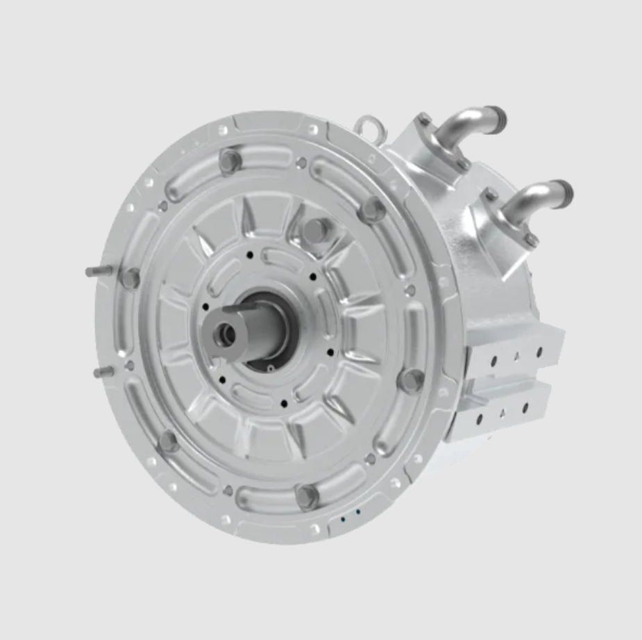
I model the permanent magnet synchronous motor in the rotor reference frame because this frame removes the time-varying inductance caused by rotor rotation. In the dq frame, the voltage equations are $$ v_d = R_s i_d + L_d \frac{di_d}{dt} – \omega_e L_q i_q $$ and $$ v_q = R_s i_q + L_q \frac{di_q}{dt} + \omega_e \left( L_d i_d + \lambda_{pm} \right) $$ where \( v_d \) and \( v_q \) are stator voltages, \( i_d \) and \( i_q \) are stator currents, \( R_s \) is stator resistance, \( L_d \) and \( L_q \) are d-axis and q-axis inductances, and \( \lambda_{pm} \) is permanent magnet flux linkage. The electromagnetic torque of the permanent magnet synchronous motor is $$ T_e = \frac{3}{2} p \left[ \lambda_{pm} i_q + \left( L_d – L_q \right) i_d i_q \right]. $$ For a surface-mounted permanent magnet synchronous motor, \( L_d \) and \( L_q \) are nearly equal, so the reluctance torque term is small. For an interior permanent magnet synchronous motor, \( L_d < L_q \), and I can exploit reluctance torque to improve efficiency and field-weakening capability. The mechanical dynamics are $$ J \frac{d\omega_m}{dt} = T_e – T_L – B \omega_m $$ where \( J \) is inertia, \( T_L \) is load torque, and \( B \) is viscous friction. These equations are the foundation for every model-based sensorless method I discuss.
Why the Permanent Magnet Synchronous Motor Suits Electric Vehicles. I find several advantages especially relevant to electric vehicle traction. First, the permanent magnet synchronous motor has high power density. It can deliver high torque from a compact and lightweight package. Second, it maintains high efficiency over a wide speed range because the rotor flux is produced by permanent magnets rather than by an additional excitation current. Third, it has fast dynamic response because torque is approximately proportional to q-axis current when the d-axis current is controlled appropriately. Fourth, it has good overload capability for short periods, which helps during launch, overtaking, and hill climbing. Fifth, it can be controlled with field-oriented control, direct torque control, or model predictive control, all of which benefit from accurate rotor position information. These advantages explain why the permanent magnet synchronous motor dominates many electric vehicle traction applications.
| Electric Vehicle Requirement | Permanent Magnet Synchronous Motor Characteristic | Benefit I Observe |
|---|---|---|
| High torque at low speed | High air-gap flux from permanent magnets | Strong launch and gradeability |
| High efficiency over wide speed range | No rotor copper loss and controllable d-axis current | Longer driving range and lower thermal load |
| Compact packaging | High torque density and power density | Smaller drivetrain volume and lower mass |
| Fast torque response | Torque controlled mainly by q-axis current | Better vehicle dynamics and traction control |
| Reliability under harsh conditions | Robust stator and rotor construction | Lower maintenance and higher availability |
| Field weakening for high speed | Negative d-axis current reduces flux linkage | Wide constant-power speed range |
I also compare the permanent magnet synchronous motor with other candidate machines because electric vehicle design always involves trade-offs. An induction motor has lower cost and no permanent magnet material risk, but it usually has lower efficiency and lower power density. A switched reluctance motor has a simple and robust rotor without magnets, but it has higher torque ripple and acoustic noise. A permanent magnet synchronous motor therefore offers an attractive balance for passenger and commercial electric vehicles, provided that sensorless control can be made reliable. This is exactly why I concentrate on the permanent magnet synchronous motor and its sensorless control methods.
| Machine Type | Power Density | Efficiency | Sensorless Difficulty | Typical Electric Vehicle Role |
|---|---|---|---|---|
| Permanent magnet synchronous motor | High | High | Moderate to high, especially at low speed | Main traction motor |
| Induction motor | Medium | Medium to high | Moderate because rotor flux is observable | Traction motor in some platforms |
| Switched reluctance motor | Medium to high | Medium | High because of strong nonlinearity | Specialized or low-cost traction |
| Brushless direct-current motor | Medium | Medium to high | Moderate but often uses Hall sensors | Light electric vehicles and auxiliary drives |
Principle of Sensorless Control. I define sensorless control as the estimation of rotor position and speed from measured electrical quantities, such as phase currents, direct-current bus voltage, inverter switching states, and sometimes temperature. The permanent magnet synchronous motor is observable through its back electromotive force, its magnetic saliency, or both. Back electromotive force is proportional to speed, so it provides strong information at medium and high speed. Magnetic saliency exists because the d-axis and q-axis inductances differ, and it provides information even at standstill. The challenge is to combine these sources so that the permanent magnet synchronous motor can be controlled from zero speed to maximum speed without a position sensor. I classify the methods into model-based back electromotive force methods, saliency-based high-frequency injection methods, nonlinear observer methods, model reference adaptive methods, stochastic filter methods, and intelligent estimation methods.
| Sensorless Method | Physical Basis | Best Speed Region | Main Strength | Main Weakness |
|---|---|---|---|---|
| Back electromotive force integration | Rotor flux linkage | Medium and high speed | Simple and intuitive | Poor at low speed and sensitive to resistance |
| Sliding mode observer | Current error and equivalent control | Medium and high speed | Strong robustness | Chattering and filtering delay |
| Model reference adaptive system | Reference and adjustable model mismatch | Medium and high speed | Moderate implementation cost | Parameter sensitivity and tuning effort |
| Extended Kalman filter | Stochastic state estimation | Wide speed range with correct model | Noise handling and covariance tuning | High computation and model dependence |
| High-frequency injection | Magnetic saliency | Zero and low speed | Position information at standstill | Audible noise, losses, and signal processing burden |
| Intelligent estimation | Data-driven mapping | Application dependent | Potential nonlinear compensation | Training data, generalization, and certification |
Back Electromotive Force Methods. I start with the back electromotive force because it is the most direct route for the permanent magnet synchronous motor. In the stationary alpha-beta frame, the back electromotive force components are $$ e_\alpha = -\omega_e \lambda_{pm} \sin \theta_e $$ and $$ e_\beta = \omega_e \lambda_{pm} \cos \theta_e. $$ The rotor electrical angle can therefore be extracted from $$ \theta_e = \tan^{-1} \left( \frac{-e_\alpha}{e_\beta} \right). $$ If I measure phase voltages and currents, I can write $$ v_\alpha = R_s i_\alpha + L_s \frac{di_\alpha}{dt} + e_\alpha $$ and $$ v_\beta = R_s i_\beta + L_s \frac{di_\beta}{dt} + e_\beta. $$ I then estimate the stator flux linkage by integration: $$ \psi_\alpha = \int \left( v_\alpha – R_s i_\alpha \right) dt $$ and $$ \psi_\beta = \int \left( v_\beta – R_s i_\beta \right) dt. $$ For the permanent magnet synchronous motor, the rotor flux linkage components satisfy $$ \psi_\alpha = L_s i_\alpha + \lambda_{pm} \cos \theta_e $$ and $$ \psi_\beta = L_s i_\beta + \lambda_{pm} \sin \theta_e. $$ Hence I can estimate the electrical angle as $$ \hat{\theta}_e = \tan^{-1} \left( \frac{\psi_\beta – L_s i_\beta}{\psi_\alpha – L_s i_\alpha} \right). $$ This method is attractive because it is easy to understand and requires limited computation. However, I have found that pure integration drifts due to direct-current offset, resistance error, and inverter nonlinearity. At low speed, the back electromotive force amplitude is very small, so the signal-to-noise ratio becomes poor. I therefore regard the back electromotive force method as a medium-speed and high-speed solution, not as a complete standstill solution for the permanent magnet synchronous motor.
I express the signal-to-noise challenge quantitatively. The back electromotive force amplitude is approximately $$ |e| = \omega_e \lambda_{pm}. $$ The signal-to-noise ratio in decibels can be written as $$ \mathrm{SNR} = 20 \log_{10} \left( \frac{|e|}{|n|} \right) $$ where \( n \) represents noise and disturbance. Because \( |e| \) falls linearly with speed, a permanent magnet synchronous motor at very low speed produces a very small back electromotive force. This is the central reason why sensorless control at zero speed and low speed requires saliency-based excitation rather than back electromotive force observation alone.
Sliding Mode Observer. I use a sliding mode observer because it provides robustness against parameter variation and external disturbance. For the permanent magnet synchronous motor, I can build a current observer in the alpha-beta frame: $$ \frac{d\hat{i}_\alpha}{dt} = -\frac{R_s}{L_s} \hat{i}_\alpha + \frac{1}{L_s} v_\alpha – \frac{1}{L_s} k \operatorname{sign} \left( \hat{i}_\alpha – i_\alpha \right) $$ and $$ \frac{d\hat{i}_\beta}{dt} = -\frac{R_s}{L_s} \hat{i}_\beta + \frac{1}{L_s} v_\beta – \frac{1}{L_s} k \operatorname{sign} \left( \hat{i}_\beta – i_\beta \right). $$ I define the sliding surface as $$ s_\alpha = \hat{i}_\alpha – i_\alpha $$ and $$ s_\beta = \hat{i}_\beta – i_\beta. $$ When the observer reaches the sliding surface, the equivalent switching signal contains the back electromotive force information. I can extract $$ \hat{e}_\alpha = k \operatorname{sign} \left( s_\alpha \right)_{\mathrm{eq}} $$ and $$ \hat{e}_\beta = k \operatorname{sign} \left( s_\beta \right)_{\mathrm{eq}}. $$ Then I estimate position by $$ \hat{\theta}_e = \tan^{-1} \left( \frac{-\hat{e}_\alpha}{\hat{e}_\beta} \right). $$ In practice, I prefer a phase-locked loop to reduce noise. I define the angle error signal as $$ \Delta \theta = -\hat{e}_\alpha \cos \hat{\theta}_e – \hat{e}_\beta \sin \hat{\theta}_e. $$ A proportional-integral controller then yields $$ \hat{\omega}_e = K_p \Delta \theta + K_i \int \Delta \theta \, dt. $$ I integrate \( \hat{\omega}_e \) to obtain \( \hat{\theta}_e \). The sliding mode observer is robust, but it produces chattering. Chattering causes current ripple, acoustic noise, and estimation error. I mitigate it with boundary layers, low-pass filters, super-twisting algorithms, or higher-order sliding modes. For the permanent magnet synchronous motor in an electric vehicle, the sliding mode observer is a strong candidate for medium and high speed, but I must design the chattering suppression carefully.
| Sliding Mode Observer Design Factor | Effect on Permanent Magnet Synchronous Motor Control | Mitigation I Apply |
|---|---|---|
| Switching gain | Too low reduces robustness; too high increases chattering | Adaptive gain based on current error |
| Boundary layer | Reduces chattering but introduces estimation lag | Variable boundary layer near zero error |
| Low-pass filter | Removes high-frequency switching noise | Phase compensation for filter delay |
| Phase-locked loop bandwidth | Trade-off between noise rejection and dynamic response | Gain scheduling with speed |
| Inverter dead time | Distorts voltage and creates angle error | Dead-time compensation and voltage feedback |
Model Reference Adaptive System. I also evaluate the model reference adaptive system for the permanent magnet synchronous motor. The idea is to use the actual machine as a reference model and an adjustable model containing estimated speed or position. The error between the reference and adjustable model drives an adaptation law. In the alpha-beta frame, I can write the current model as $$ \frac{di_\alpha}{dt} = -\frac{R_s}{L_s} i_\alpha + \frac{1}{L_s} v_\alpha – \frac{1}{L_s} e_\alpha $$ and $$ \frac{di_\beta}{dt} = -\frac{R_s}{L_s} i_\beta + \frac{1}{L_s} v_\beta – \frac{1}{L_s} e_\beta. $$ The adjustable model uses \( \hat{\omega}_e \) and \( \hat{\theta}_e \). A common adaptation law for speed is $$ \hat{\omega}_e = K_p \left( i_\alpha \hat{e}_\beta – i_\beta \hat{e}_\alpha \right) + K_i \int \left( i_\alpha \hat{e}_\beta – i_\beta \hat{e}_\alpha \right) dt. $$ This structure is simpler than some nonlinear observers and can work well at medium and high speed. However, the permanent magnet synchronous motor parameters change with temperature and magnetic saturation. If \( R_s \) or \( \lambda_{pm} \) is incorrect, the estimated speed contains steady-state error. I therefore combine model reference adaptive systems with online parameter identification or with robust control terms. I rarely rely on a model reference adaptive system alone for the full speed range of an electric vehicle.
High-Frequency Injection. For zero-speed and low-speed operation, I use high-frequency injection because it exploits magnetic saliency. In an interior permanent magnet synchronous motor, the d-axis and q-axis inductances differ. When I inject a high-frequency voltage signal into the stator, the current response contains rotor position information. A simplified rotating injection can be described by $$ v_{dh} = V_h \cos \left( \omega_h t \right) $$ and $$ v_{qh} = V_h \sin \left( \omega_h t \right). $$ The high-frequency current response in the stationary frame contains a negative-sequence component related to the rotor angle. I express the position-dependent current term as $$ i_{\alpha\beta,h} = I_h e^{j\omega_h t} – I_n e^{j \left( 2\theta_e – \omega_h t \right)}. $$ I then demodulate the negative-sequence component and estimate \( \theta_e \). Because the method does not depend on back electromotive force, it works at standstill. The cost is additional loss, audible noise, torque ripple, and computational burden. I must select the injection frequency, voltage amplitude, and demodulation filter carefully. For the permanent magnet synchronous motor in an electric vehicle, high-frequency injection is most useful during launch, parking, creep, and hill holding, where low-speed position accuracy is critical.
| High-Frequency Injection Choice | Advantage | Disadvantage | My Preferred Use |
|---|---|---|---|
| Rotating voltage injection | Position observability in all directions | Torque ripple and acoustic noise | Standstill and low-speed initial position detection |
| Pulsating d-axis injection | Less torque ripple in some operating points | Requires accurate current control and filters | Low-speed sensorless control of the permanent magnet synchronous motor |
| Square-wave injection | Wide bandwidth and less filter delay | Higher harmonic loss and electromagnetic interference | Fast dynamic low-speed estimation |
| Random or spread-spectrum injection | Reduces tonal noise | More complex demodulation | Passenger electric vehicles with noise constraints |
Stochastic and Nonlinear Observers. I use the extended Kalman filter when I need a systematic way to handle measurement noise and model uncertainty. I define the state vector as $$ x = \begin{bmatrix} i_d & i_q & \omega_e & \theta_e \end{bmatrix}^T. $$ The discrete nonlinear model is $$ x_{k+1} = f \left( x_k, u_k \right) + w_k $$ and the measurement model is $$ y_k = h \left( x_k \right) + v_k. $$ The prediction step is $$ \hat{x}_{k|k-1} = f \left( \hat{x}_{k-1|k-1}, u_{k-1} \right) $$ and $$ P_{k|k-1} = F_{k-1} P_{k-1|k-1} F_{k-1}^T + Q_{k-1}. $$ The update step is $$ K_k = P_{k|k-1} H_k^T \left( H_k P_{k|k-1} H_k^T + R_k \right)^{-1}, $$ $$ \hat{x}_{k|k} = \hat{x}_{k|k-1} + K_k \left( y_k – h \left( \hat{x}_{k|k-1} \right) \right), $$ and $$ P_{k|k} = \left( I – K_k H_k \right) P_{k|k-1}. $$ The extended Kalman filter can estimate position and speed simultaneously, but it is computationally intensive and depends on covariance tuning. I find that it can perform well for the permanent magnet synchronous motor if the noise statistics are realistic, but it is not always the best choice for low-cost embedded controllers. Unscented Kalman filters and cubature Kalman filters can improve nonlinear handling at additional computation cost.
Challenges in Electric Vehicle Applications. I now turn to the practical challenges that dominate my engineering work. The first challenge is low-speed performance. At low speed, the back electromotive force of the permanent magnet synchronous motor is small, so the observer signal-to-noise ratio is low. Inverter dead time, switch voltage drops, current measurement offset, and analog-to-digital quantization become significant relative to the useful signal. The second challenge is parameter variation. Stator resistance changes with temperature. Permanent magnet flux linkage changes with temperature and aging. Inductance changes with current because of magnetic saturation. These variations cause model mismatch and steady-state estimation error. The third challenge is electromagnetic interference. The traction inverter switches at high frequency, and the permanent magnet synchronous motor is exposed to common-mode voltage, cable ringing, and radiated noise. These disturbances corrupt current and voltage measurements and degrade observer accuracy. The fourth challenge is real-time computation. Sensorless algorithms must execute within the current control loop, often at tens of microseconds. The fifth challenge is safety and fault tolerance. An electric vehicle must behave safely if estimation quality degrades, if a current sensor fails, or if the inverter enters an overmodulation region.
| Challenge | Physical Cause | Effect on the Permanent Magnet Synchronous Motor | Severity |
|---|---|---|---|
| Low-speed estimation error | Small back electromotive force and low signal-to-noise ratio | Poor launch, creep, hill holding, and stop-start behavior | High |
| Parameter drift | Temperature, aging, and magnetic saturation | Angle error, torque error, efficiency loss | High |
| Electromagnetic interference | Pulse-width modulation, common-mode voltage, cable coupling | Noisy measurements and observer instability | Medium to high |
| Inverter nonlinearity | Dead time, voltage drop, switching delay | Voltage distortion and position offset | High at low speed |
| Computational delay | Digital sampling and execution time | Phase lag and reduced phase margin | Medium |
| Mode transition | Switching between low-speed and high-speed observers | Transient angle error and torque disturbance | Medium to high |
I quantify parameter effects because this helps me design compensation. The stator resistance can be written as $$ R_s \left( T \right) = R_{s0} \left[ 1 + \alpha_R \left( T – T_0 \right) \right] $$ where \( \alpha_R \) is the temperature coefficient and \( T_0 \) is a reference temperature. The permanent magnet flux linkage can be written as $$ \lambda_{pm} \left( T \right) = \lambda_{pm0} \left[ 1 + \alpha_\lambda \left( T – T_0 \right) \right] $$ where \( \alpha_\lambda \) is usually negative for common permanent magnet materials. The inductances depend on current: $$ L_d = L_d \left( i_d, i_q \right) $$ and $$ L_q = L_q \left( i_d, i_q \right). $$ A torque error caused by parameter mismatch can be approximated by $$ \Delta T_e = \frac{3}{2} p \left[ \Delta \lambda_{pm} i_q + \Delta \left( L_d – L_q \right) i_d i_q \right]. $$ This expression shows why I cannot ignore parameter variation in a high-performance permanent magnet synchronous motor drive. Even a modest flux error changes torque calibration and can cause the vehicle controller to command incorrect current references.
Electromagnetic interference is another issue I cannot treat casually. The inverter applies high-frequency pulse-width modulation, and the cables between inverter and motor behave like transmission lines. Common-mode voltage can produce shaft voltage and bearing current. Differential-mode noise corrupts phase current measurement. If I use a sliding mode observer, the switching term can amplify noise. If I use a Kalman filter, incorrect noise covariance can cause divergence. If I use high-frequency injection, the injected signal itself becomes a source of electromagnetic interference. I therefore apply a combination of hardware and software measures: shielded cables, common-mode chokes, differential current sensing, analog anti-aliasing filters, synchronized sampling, random pulse-width modulation, and robust digital filters. I also verify the sensorless algorithm under realistic electromagnetic compatibility conditions rather than only in an ideal simulation.
Solution Strategies. My first strategy is hybrid estimation. I use high-frequency injection for zero and low speed, and I use back electromotive force or sliding mode observation for medium and high speed. I blend the two estimates with a speed-dependent weight. I define a transition variable $$ \alpha \left( \omega_e \right) = \mathrm{saturate} \left( \frac{\omega_e – \omega_{\mathrm{low}}}{\omega_{\mathrm{high}} – \omega_{\mathrm{low}}} \right) $$ where \( \omega_{\mathrm{low}} \) and \( \omega_{\mathrm{high}} \) define the transition band. The blended position estimate can be written as $$ \hat{\theta}_e = \alpha \hat{\theta}_{e,\mathrm{high}} + \left( 1 – \alpha \right) \hat{\theta}_{e,\mathrm{low}}. $$ I must handle angle wrapping carefully, so I often blend the sine and cosine components instead of the raw angles: $$ \hat{\theta}_e = \operatorname{atan2} \left( \alpha \sin \hat{\theta}_{e,\mathrm{high}} + \left( 1 – \alpha \right) \sin \hat{\theta}_{e,\mathrm{low}}, \alpha \cos \hat{\theta}_{e,\mathrm{high}} + \left( 1 – \alpha \right) \cos \hat{\theta}_{e,\mathrm{low}} \right). $$ This hybrid approach allows the permanent magnet synchronous motor to operate from standstill to high speed with a single controller structure.
| Operating Region | Primary Estimation Method | Secondary Support | Control Objective |
|---|---|---|---|
| Standstill and initial position | High-frequency injection | Saliency detection and polarity test | Correct initial angle and safe launch |
| Low speed | High-frequency injection or pulsating injection | Parameter adaptation and inverter compensation | Creep, hill holding, and smooth torque |
| Medium speed | Sliding mode observer or model reference adaptive system | Phase-locked loop and filtering | Efficient torque control and mode transition |
| High speed | Back electromotive force observer | Flux weakening and voltage margin control | Constant-power operation and stability |
| Regenerative braking | Hybrid observer with current sign compensation | Voltage limitation and fault detection | Safe energy recovery and brake feel |
My second strategy is advanced observer design. I replace the conventional sign function in the sliding mode observer with a super-twisting algorithm to reduce chattering. A simplified super-twisting current observer can be written as $$ \frac{d\hat{i}}{dt} = -\frac{R_s}{L_s} \hat{i} + \frac{1}{L_s} v – k_1 |s|^{1/2} \operatorname{sign} \left( s \right) + z $$ and $$ \frac{dz}{dt} = -k_2 \operatorname{sign} \left( s \right). $$ This structure maintains robustness while producing a smoother equivalent back electromotive force. I also use adaptive sliding mode gains that increase when the estimation error grows and decrease when the system is near the sliding surface. For the permanent magnet synchronous motor, this reduces current ripple and acoustic noise without sacrificing disturbance rejection. I have also explored fixed-time observers, terminal sliding mode observers, and disturbance observers. Each method has a different trade-off between convergence speed, chattering, and implementation complexity.
My third strategy is online parameter identification. I use recursive least squares to estimate stator resistance, permanent magnet flux linkage, and inductances. The recursive least squares update is $$ \hat{\theta}_k = \hat{\theta}_{k-1} + K_k \left( y_k – \phi_k^T \hat{\theta}_{k-1} \right), $$ $$ K_k = \frac{P_{k-1} \phi_k}{\lambda + \phi_k^T P_{k-1} \phi_k}, $$ and $$ P_k = \frac{1}{\lambda} \left( I – K_k \phi_k^T \right) P_{k-1}, $$ where \( \lambda \) is the forgetting factor. The parameter vector may include \( R_s \), \( \lambda_{pm} \), \( L_d \), and \( L_q \). Because not all parameters are identifiable at every operating point, I use injection or excitation when necessary. For example, I can estimate \( R_s \) at low speed with direct-current injection, and I can estimate \( \lambda_{pm} \) at medium speed with q-axis current. I also use temperature measurements and thermal models to constrain the identification. This improves the accuracy of the permanent magnet synchronous motor sensorless controller over the full vehicle lifetime.
| Parameter | Main Variation Source | Identification Signal | Compensation Method |
|---|---|---|---|
| Stator resistance \( R_s \) | Temperature and cable resistance | Direct-current or low-frequency injection | Recursive least squares and thermal model |
| Permanent magnet flux \( \lambda_{pm} \) | Temperature and aging | Medium-speed q-axis operation | Online flux observer and look-up table |
| d-axis inductance \( L_d \) | Magnetic saturation | High-frequency injection | Current-dependent look-up table |
| q-axis inductance \( L_q \) | Magnetic saturation and cross-coupling | High-frequency injection and load steps | Multidimensional look-up table |
| Inverter voltage error | Dead time and switch drop | Current polarity and terminal voltage measurement | Dead-time compensation and voltage observer |
My fourth strategy is robust filtering and disturbance rejection. I use a phase-locked loop with adaptive bandwidth. At low speed, I reduce the bandwidth to reject noise. At high speed, I increase the bandwidth to improve dynamic response. I also use notch filters to remove specific harmonic disturbances caused by inverter dead time and current measurement offset. I define the estimated speed error as $$ \omega_{\mathrm{err}} = \omega_e – \hat{\omega}_e. $$ A disturbance observer can estimate the lumped disturbance \( d \) as $$ \hat{d} = \left( K_{p,d} + \frac{K_{i,d}}{s} \right) \omega_{\mathrm{err}}. $$ I then feed \( \hat{d} \) forward to the current controller to improve disturbance rejection. This is especially useful during vehicle load changes, road grade changes, and regenerative braking transitions. For the permanent magnet synchronous motor, robust filtering must be designed together with the current loop because delay in the observer can destabilize the speed loop.
My fifth strategy is electromagnetic interference mitigation. I use differential-mode and common-mode filters, shielded motor cables, and careful grounding. I synchronize analog-to-digital conversion with pulse-width modulation to avoid switching noise. I use oversampling and averaging when the control bandwidth permits. I apply random pulse-width modulation or spread-spectrum modulation to reduce tonal noise. I also validate the permanent magnet synchronous motor sensorless controller in a chassis dynamometer or hardware-in-the-loop environment with realistic inverter and cable models. In my experience, software-only improvement cannot fully compensate for poor electromagnetic compatibility design. The hardware and software must be co-designed.
| Solution Strategy | Target Challenge | Implementation Cost | Expected Benefit |
|---|---|---|---|
| Hybrid low-speed and high-speed observer | Limited speed range of single method | Medium | Full-speed sensorless operation |
| Super-twisting sliding mode | Chattering and disturbance | Medium | Lower ripple and stronger robustness |
| Online parameter identification | Temperature and saturation | High | Accurate angle and torque over lifetime |
| Adaptive phase-locked loop | Noise and dynamic trade-off | Low | Better noise rejection and response |
| Electromagnetic compatibility design | Measurement corruption | Medium to high | Stable observer and safer operation |
| Fault detection and limp-home mode | Sensor or observer failure | Medium | Functional safety and availability |
Implementation and Evaluation. I evaluate sensorless control for the permanent magnet synchronous motor with several quantitative metrics. The position error is $$ \theta_{\mathrm{err}} = \theta_e – \hat{\theta}_e $$ after angle unwrapping. The speed error is $$ \omega_{\mathrm{err}} = \omega_e – \hat{\omega}_e. $$ I compute the root-mean-square position error as $$ \mathrm{RMSE}_\theta = \sqrt{\frac{1}{N} \sum_{i=1}^{N} \theta_{\mathrm{err},i}^2}. $$ I also measure torque ripple, current total harmonic distortion, efficiency, and response time. The efficiency of the permanent magnet synchronous motor drive can be written as $$ \eta = \frac{P_{\mathrm{mech}}}{P_{\mathrm{elec}}} \times 100\% $$ where \( P_{\mathrm{mech}} \) is mechanical output power and \( P_{\mathrm{elec}} \) is electrical input power. I compare sensorless operation with sensored operation to quantify the penalty. In a well-designed system, the penalty at medium and high speed can be small, but at low speed the penalty can be significant unless high-frequency injection and parameter compensation are used.
| Metric | Definition | Typical Target for Electric Vehicle Traction | Main Influencing Factor |
|---|---|---|---|
| Position error | Difference between actual and estimated electrical angle | Small enough to avoid torque loss and current distortion | Observer bandwidth, parameter accuracy, noise |
| Speed error | Difference between actual and estimated electrical speed | Low steady-state error and fast transient recovery | Phase-locked loop tuning and load disturbance |
| Torque ripple | Periodic torque fluctuation | Low enough for passenger comfort | Angle error, current harmonics, cogging torque |
| Current total harmonic distortion | Harmonic content in phase current | Low to reduce loss and noise | Inverter nonlinearity and observer noise |
| Efficiency | Mechanical output divided by electrical input | High over wide speed and load range | Parameter mismatch, flux weakening, thermal state |
| Response time | Time to recover after torque command or load step | Short enough for vehicle dynamics | Observer convergence and controller gain |
I test the permanent magnet synchronous motor sensorless controller in a sequence of operating conditions. I start with standstill initial position detection. I then test low-speed creep, hill holding, and reverse motion. I continue with medium-speed acceleration, high-speed field weakening, and regenerative braking. I also test parameter variation by heating the machine and by changing the direct-current bus voltage. I inject electromagnetic interference through the cable and observe whether the observer remains stable. I test fault conditions such as current sensor offset, phase loss, and inverter dead-time mismatch. Finally, I evaluate the transition between low-speed injection and high-speed back electromotive force observation. A smooth transition is essential because an angle jump during transition can produce torque shock, current overshoot, or vehicle jerk.
Transient Behavior and Stability. I pay special attention to stability because sensorless control couples the observer with the current controller and speed controller. The estimated angle error affects torque production, and torque production affects speed, which in turn affects the observer. This closed-loop interaction can create oscillations if the observer bandwidth is too low or too high. I use small-signal analysis around an operating point. The torque sensitivity to angle error is approximately $$ \frac{\partial T_e}{\partial \theta_{\mathrm{err}}} \approx -\frac{3}{2} p \lambda_{pm} i_q \sin \theta_{\mathrm{err}} – \frac{3}{2} p \left( L_d – L_q \right) i_d i_q \cos \theta_{\mathrm{err}}. $$ For small errors, this becomes $$ \frac{\partial T_e}{\partial \theta_{\mathrm{err}}} \approx -\frac{3}{2} p \lambda_{pm} i_q. $$ This relation shows that a given angle error causes a torque error proportional to q-axis current. At high load, the same angle error produces a larger torque error. I therefore make the observer bandwidth and the current controller bandwidth compatible. I also limit the speed controller bandwidth so that it does not amplify observer noise.
I also consider the effect of voltage saturation. At high speed, the inverter reaches its voltage limit, and field weakening is required. The available voltage for current control decreases, so the observer has less excitation. I use a voltage margin controller and a flux-weakening controller. The voltage constraint can be written as $$ v_d^2 + v_q^2 \le V_{\mathrm{max}}^2 $$ where \( V_{\mathrm{max}} \) depends on the direct-current bus voltage and modulation strategy. The current constraint is $$ i_d^2 + i_q^2 \le I_{\mathrm{max}}^2. $$ The maximum torque per ampere trajectory and the field-weakening trajectory must be coordinated with the sensorless observer. If the observer requires voltage injection at high speed, it may conflict with the voltage limit. Therefore, I disable injection when it is not needed and rely on back electromotive force observation in the high-speed region.
| Operating Condition | Main Constraint | Observer Risk | Controller Action |
|---|---|---|---|
| Standstill | No back electromotive force | No position observability without saliency | Inject high-frequency signal and detect saliency |
| Low speed | Low signal-to-noise ratio | Angle noise and drift | Use injection, increase filtering, compensate dead time |
| Medium speed | Parameter mismatch | Steady-state angle error | Use robust observer and online identification |
| High speed | Voltage limit and field weakening | Reduced observer excitation | Use back electromotive force observer and voltage margin control |
| Regenerative braking | Current sign reversal and voltage rise | Dead-time compensation error | Use sign-aware compensation and safe torque limits |
Vehicle-Level Integration. I integrate the permanent magnet synchronous motor sensorless controller with the vehicle control unit, the battery management system, and the inverter controller. The vehicle control unit sends a torque request. The motor controller translates that request into d-axis and q-axis current references. The sensorless observer provides rotor position and speed. The inverter applies the voltage vector. The battery management system limits power based on state of charge, temperature, and voltage. If the observer confidence is low, the controller must reduce torque or enter a limp-home mode. I define an observer confidence index based on current error, back electromotive force magnitude, signal-to-noise ratio, and parameter consistency. When confidence falls below a threshold, I switch to a safer control mode. This is important for functional safety because an uncontrolled permanent magnet synchronous motor can produce unintended torque.
I also consider noise, vibration, and harshness. High-frequency injection can produce audible noise in the passenger cabin. Sliding mode chattering can produce current ripple and tonal noise. Dead-time compensation errors can produce torque ripple. I therefore use spread-spectrum injection, randomized switching, and adaptive filtering. I also shape the torque command with a rate limiter and a notch filter at the resonance frequency of the drivetrain. For the permanent magnet synchronous motor, sensorless control must not compromise the driving experience. A small angle error may be acceptable for efficiency, but it may be unacceptable if it creates vibration or torque shock.
| Vehicle-Level Requirement | Sensorless Control Implication | Design Measure |
|---|---|---|
| Safety | Prevent unintended torque and loss of control | Observer confidence monitoring and torque limiting |
| Comfort | Minimize torque ripple and acoustic noise | Random injection, filtering, and smooth mode transition |
| Efficiency | Reduce losses from estimation error and injection | Disable injection when not needed and adapt current references |
| Durability | Protect inverter and motor from overheating | Thermal monitoring and current derating |
| Availability | Continue operation after partial faults | Fault detection and limp-home strategy |
| Cost | Remove position sensor and reduce wiring | Embedded observer with limited computation |
Comparison of Practical Design Choices. I have compared several design choices for the permanent magnet synchronous motor in electric vehicles. If cost is the primary concern, I choose a medium-speed sliding mode observer with a simple phase-locked loop and no high-frequency injection. This reduces sensor cost but limits low-speed performance. If low-speed performance is critical, I add high-frequency injection and a saliency-based observer. If parameter robustness is critical, I add online identification. If functional safety is critical, I add redundancy through a model-based observer and a signal-based monitor. If computational resources are abundant, I use an extended Kalman filter or an unscented Kalman filter. The best design depends on the vehicle segment, the motor saliency, the inverter switching frequency, the available microcontroller, and the safety requirements.
| Design Priority | Recommended Sensorless Architecture | Trade-Off | Suitable Electric Vehicle Application |
|---|---|---|---|
| Lowest cost | Back electromotive force observer with phase-locked loop | Poor standstill and low-speed performance | Low-speed requirement not critical |
| Wide speed range | High-frequency injection plus sliding mode observer | Higher computation and acoustic noise | Passenger electric vehicle traction |
| High robustness | Super-twisting sliding mode plus online identification | Complex tuning and computation | Commercial vehicle and harsh environment |
| High accuracy | Extended Kalman filter with parameter adaptation | High processor load and covariance tuning | Premium electric vehicle with strong processor |
| Functional safety | Hybrid observer with independent monitor and confidence index | Development effort and validation cost | Safety-critical traction system |
Future Directions. I see several future directions for sensorless control of the permanent magnet synchronous motor. The first is the use of artificial intelligence and machine learning to compensate nonlinear effects such as magnetic saturation, inverter dead time, and cross-coupling. A neural network or Gaussian process can learn a correction map from measured data. However, I remain cautious because certification and generalization are difficult. The second direction is digital twin technology. A digital twin of the permanent magnet synchronous motor can run in parallel with the real machine and provide parameter updates, fault detection, and remaining useful life estimation. The third direction is wide-bandgap inverter technology. Silicon carbide and gallium nitride devices switch faster and reduce losses, but they also increase electromagnetic interference and voltage reflection. Sensorless observers must be redesigned for these conditions. The fourth direction is edge computing and cloud-based parameter learning. The fifth direction is functional safety standardization, where sensorless control is treated as a safety-related function with defined integrity levels. I believe these directions will shape the next generation of electric vehicle traction controllers.
| Future Technology | Potential Benefit for the Permanent Magnet Synchronous Motor | Key Challenge |
|---|---|---|
| Machine learning compensation | Improved nonlinear mapping and parameter adaptation | Data dependency, verification, and certification |
| Digital twin | Continuous parameter estimation and fault prediction | Model fidelity and real-time coupling |
| Wide-bandgap inverter | Higher efficiency and power density | Stronger electromagnetic interference and insulation stress |
| Edge and cloud computing | Adaptive tuning and fleet-level learning | Cybersecurity, latency, and data privacy |
| Functional safety integration | Certifiable sensorless control | Diagnostic coverage and fault-tolerant architecture |
Conclusion. In my first-person engineering assessment, sensorless control of the permanent magnet synchronous motor is a key enabling technology for electric vehicles. I have explained why the permanent magnet synchronous motor offers high power density, high efficiency, and excellent dynamic performance. I have presented the dq-frame equations, torque equations, back electromotive force relations, flux linkage observers, sliding mode observers, model reference adaptive systems, high-frequency injection, and Kalman filter formulations. I have also examined the main challenges: low-speed signal-to-noise ratio, parameter variation, inverter nonlinearity, electromagnetic interference, computational delay, and mode transition. I have proposed hybrid estimation, advanced sliding mode design, online parameter identification, adaptive filtering, electromagnetic compatibility co-design, and vehicle-level safety integration as practical solutions. I have used tables to compare methods, operating regions, design priorities, and future technologies. The permanent magnet synchronous motor will remain central to electric vehicle traction, and sensorless control will continue to improve in accuracy, robustness, and safety. In my view, the most promising path is not a single universal observer but a carefully coordinated hybrid architecture that uses saliency at low speed, back electromotive force at high speed, and continuous parameter adaptation throughout the life of the permanent magnet synchronous motor. Through this approach, I believe electric vehicles can achieve lower cost, higher reliability, and better overall performance without relying on a mechanical rotor position sensor.