
I have focused my research on the thermal management of a PMSM electric motor, because excessive heat generation under high-speed operation directly degrades performance, reduces service life, and can even cause irreversible demagnetization. In this work, I propose an improved multi-objective nonlinear magnetic-thermal coupling iterative calculation method. My method accounts for the temperature dependence of copper winding resistivity and permanent magnet magnetic properties, as well as the influence of permanent magnet demagnetization on the electromagnetic field. I verify my approach on a 40 kW automotive PMSM electric motor, and then I use orthogonal experiments to optimize the cooling channel design. The following sections present my complete analysis, including the physical model, electromagnetic characteristics, loss calculations, coupling iterations, experimental validation, and flow channel optimization.
1 Physical Model and Parameters of the PMSM Electric Motor
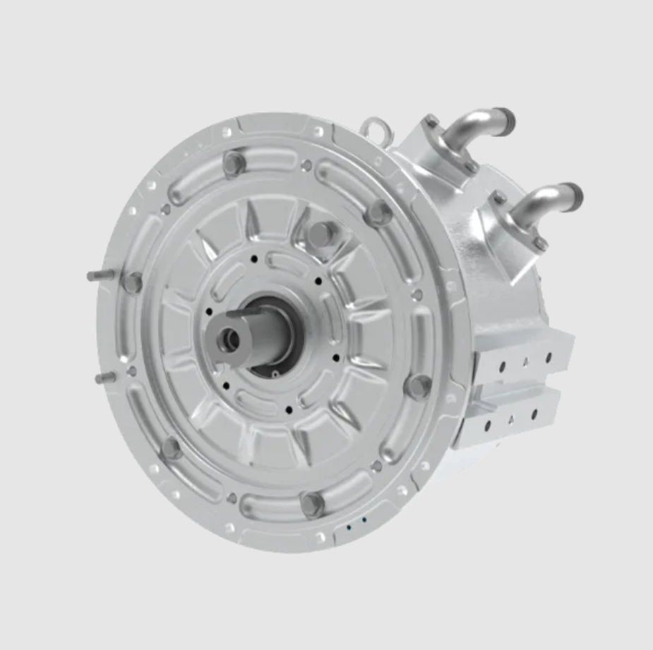
The PMSM electric motor I study is a 40 kW, 8100 r/min interior permanent magnet synchronous motor. It uses an 8-pole, 48-slot double-layer winding configuration, and the rotor has a built-in “double V” structure. This design provides high torque density and good flux-weakening capability, which are essential for electric vehicle applications. The main parameters of the PMSM electric motor are summarized in Table 1.
| Parameter | Value |
|---|---|
| Rated power | 40 kW |
| Rated speed | 8100 r/min |
| Rated torque | 48 Nm |
| Peak speed | 12000 r/min |
| Peak torque | 32 Nm |
| Stator outer diameter | 180 mm |
| Stator inner diameter | 120 mm |
| Air gap | 0.6 mm |
Due to the symmetry of the PMSM electric motor, I use a 1/8 model for the two-dimensional transient electromagnetic field calculation. This reduces computational cost while preserving accuracy. The material parameters used in the thermal model are listed in Table 2.
| Material | Density (kg/m³) | Specific heat (J/(kg·K)) | Thermal conductivity (W/(m·K)) |
|---|---|---|---|
| Housing | 2680 | 963 | 150 |
| Shaft | 7850 | 460 | 48 |
| Insulation slot | 8030 | 502.48 | 0.22 |
| Winding | 8978 | 390 | 401 |
| Stator/rotor core (radial) | 8030 | 502.48 | 39 |
| Stator/rotor core (axial) | 8030 | 502.48 | 4.43 |
| Coolant | 1073.3 | 3281 | 0.38 |
| Permanent magnet | 8030 | 502.48 | 9 |
2 Electromagnetic Characteristics of the PMSM Electric Motor
2.1 No-Load Characteristics
I first analyze the no-load magnetic flux density distribution and the magnetic field line distribution of the PMSM electric motor at rated speed. The flux density is uniformly distributed, and the maximum value is concentrated in the rotor bridge region. This indicates that the magnetic circuit design is reasonable. The magnetic field lines are periodically distributed, and the flux barriers play a significant role. The air-gap flux density is approximately sinusoidal, and its Fourier decomposition shows that the harmonic content is well controlled. The maximum value is about 0.8 T, which means the magnetic flux utilization is high.
The air-gap flux density can be expressed as a Fourier series:
$$B_g(\theta) = \sum_{n=1}^{\infty} B_n \sin(n\theta + \phi_n)$$
where \(B_n\) is the amplitude of the \(n\)-th harmonic, \(\theta\) is the mechanical angle, and \(\phi_n\) is the phase angle. The fundamental component dominates, which is desirable for smooth torque production in the PMSM electric motor.
2.2 Load Characteristics
I calculate the torque and power characteristics of the PMSM electric motor under two operating conditions: 40 kW, 8100 r/min, 48 Nm and 40 kW, 12000 r/min, 32 Nm. The torque remains stable with small ripple, and the output power meets the design requirements. This confirms that the electromagnetic design of the PMSM electric motor is sound.
The electromagnetic torque of the PMSM electric motor can be written as:
$$T_e = \frac{3}{2} p \left[ \psi_{PM} i_q + (L_d – L_q) i_d i_q \right]$$
where \(p\) is the pole pair number, \(\psi_{PM}\) is the permanent magnet flux linkage, \(L_d\) and \(L_q\) are the d-axis and q-axis inductances, and \(i_d\) and \(i_q\) are the d-axis and q-axis currents. This equation shows that the reluctance torque contributes to the total torque in an interior PMSM electric motor.
3 Loss Calculation of the PMSM Electric Motor
The losses in the PMSM electric motor mainly include stator and rotor core losses, permanent magnet eddy current losses, and winding copper losses. Mechanical losses are neglected because they have a much smaller effect on the temperature field. I calculate each loss component as follows.
3.1 Core Loss
The core loss is composed of hysteresis loss, eddy current loss, and excess loss. I use the Bertotti model:
$$P_{Fe} = k_h f B_m^a + k_e f^2 B_m^2 + k_a f^{1.5} B_m^{1.5}$$
where \(B_m\) is the flux density amplitude, \(f\) is the magnetic field frequency, and \(k_h\), \(k_e\), and \(k_a\) are the hysteresis, eddy current, and excess loss coefficients, respectively. These coefficients are obtained by fitting the silicon steel loss curves.
3.2 Permanent Magnet Eddy Current Loss
The permanent magnet eddy current loss is calculated as:
$$P_E = \int_V \mathbf{E} \cdot \mathbf{J}_w \, dV = \int_V \frac{J_w^2}{\sigma} \, dV = \int_V \rho J_w^2 \, dV$$
where \(P_E\) is the permanent magnet loss, \(\sigma\) is the electrical conductivity, \(\mathbf{E}\) is the eddy current electric field, \(\mathbf{J}_w\) is the eddy current density, \(\rho\) is the resistivity, and \(V\) is the volume of the permanent magnet.
3.3 Winding Copper Loss
The copper loss considering temperature variation is:
$$P_{cu} = m I^2 R$$
$$R = R_0 \left[ 1 + \beta_0 (T – T_0) \right] = \frac{\rho_{za} L_z}{S} \left[ 1 + \beta_0 (T – T_0) \right]$$
where \(m\) is the number of phases, \(I\) is the RMS current, \(R_0\) is the base resistance, \(\beta_0\) is the temperature coefficient, \(L_z\) is the conductor length, \(\rho_{za}\) is the copper resistivity, \(S\) is the cross-sectional area, and \(T_0\) is the reference temperature.
The loss values for the two operating conditions are summarized in Table 3.
| Operating condition | Stator core loss (W) | Rotor core loss (W) | Eddy current loss (W) | Winding loss (W) |
|---|---|---|---|---|
| 40 kW, 8100 r/min, 48 Nm | 649.5 | 69.43 | 5.90 | 840 |
| 40 kW, 12000 r/min, 32 Nm | 848.8 | 84.71 | 4.55 | 740 |
4 Improved Multi-Objective Nonlinear Magnetic-Thermal Coupling Method
4.1 Mathematical Model of the Coupling
In my improved method, I consider the temperature dependence of both the winding resistance and the permanent magnet magnetic properties. The temperature effect on the permanent magnet is described by:
$$B_{rt1} = \left( 1 – \frac{IL}{100} \right) \left[ 1 + \frac{(t_1 – t_0) \alpha_{Br}}{100} \right] B_{rt0}$$
$$H_{ct1} = \left( 1 – \frac{IL}{100} \right) \left[ 1 + \frac{(t_1 – t_0) \alpha_{Hc}}{100} \right] H_{ct0}$$
where \(B_{rt0}\) is the remanence at \(t_0\) °C, \(\alpha_{Br}\) is the reversible temperature coefficient of remanence, \(\alpha_{Hc}\) is the temperature coefficient of coercivity, \(IL\) is the irreversible loss rate of remanence, \(t_1\) is the operating temperature, and \(H_{ct0}\) is the coercivity at \(t_0\) °C.
The temperature effect on the winding resistivity is:
$$\rho = \rho_0 \left[ 1 + \beta_0 (T – T_0) \right]$$
where \(\rho_0\) is the base resistivity at the reference temperature.
4.2 Iterative Mechanism and Flowchart
Traditional magnetic-thermal coupling only considers the variation of copper resistivity with temperature and ignores the effect of temperature on the permanent magnet magnetic properties. However, both the copper resistivity and the permanent magnet magnetic properties are affected by temperature, and the high-temperature demagnetization of the permanent magnet affects the magnetic field and losses of the PMSM electric motor. Based on this uncertain relationship, I propose an improved multi-objective nonlinear magnetic-thermal coupling iterative calculation method.
First, based on the two-dimensional transient model of the PMSM electric motor, combined with the temperature resistance grade and simulation experience, I take the initial operating temperature of the permanent magnet as 80 °C and the stator winding resistivity as 2.19 Ω/m. I determine the B-H curve of the permanent magnet at 80 °C. After electromagnetic calculation, I obtain the first set of losses. Using the heat flux density formula:
$$J = \frac{Q}{A \cdot L}$$
where \(J\) is the heat flux density, \(Q\) is the heat dissipation per unit time, \(A\) is the effective heat dissipation area, and \(L\) is the axial length. I calculate the heat sources for the three-dimensional heat transfer model, as shown in Table 4.
| Heat source | Loss (W) | Heat flux density (W/m³) |
|---|---|---|
| Stator core loss | 649.5 | 692881.29 |
| Rotor core loss | 69.43 | 113808.81 |
| Eddy current loss | 5.90 | 64698.98 |
| Winding loss | 840 | 4003946.72 |
After the first calculation, the average temperatures of the permanent magnet and the stator winding are 93.31 °C and 109 °C, respectively. Based on these values, I determine the new stator winding resistivity at 109 °C and use linear interpolation to calculate the B-H curve of the permanent magnet at 93 °C. Then I perform a new iteration of the two-dimensional transient field of the PMSM electric motor, obtaining new losses and new heat flux densities. I recalculate the three-dimensional flow-thermal coupling field. In this cycle, I perform multiple iterative calculations of the magnetic field and thermal field of the PMSM electric motor. The convergence criterion is:
$$\frac{|T_{pa}^{n+1} – T_{pa}^{n}|}{T_{pa}^{n+1}} \leq \varepsilon_1, \quad \frac{|T_{za}^{n+1} – T_{za}^{n}|}{T_{za}^{n+1}} \leq \varepsilon_2$$
where \(T_{pa}^n\) is the average temperature of the permanent magnet at iteration \(n\), \(T_{pa}^{n+1}\) is the average temperature at iteration \(n+1\), \(T_{za}^n\) is the average temperature of the stator winding at iteration \(n\), and \(T_{za}^{n+1}\) is the average temperature at iteration \(n+1\). I set \(\varepsilon_1 = \varepsilon_2 = 0.8\%\).
To accurately calculate the parameter changes during operation, I need to consider the performance degradation of the permanent magnet at high temperatures. Since existing data only provide demagnetization curves at fixed temperatures such as 80 °C, 100 °C, and 120 °C, I use linear interpolation to estimate the magnetic properties at a specific temperature:
$$\psi(B,H) = \frac{f_{x1}(B,H) – f_{x0}(B,H)}{x_1 – x_0}$$
$$f_x(B,H) = f_{x0}(B,H) + \psi(B,H)(x – x_0)$$
where \(\psi(B,H)\) is the unit difference, \(f_{x1}(B,H)\) is the B-H curve at temperature \(x_1\), \(f_{x0}(B,H)\) is the B-H curve at temperature \(x_0\), and \(f_x(B,H)\) is the B-H curve at temperature \(x\).
4.3 Coupling of Key Parameters
I consider the actual operating conditions of the PMSM electric motor: the inlet water temperature is 65 °C, the flow rate is 12 L/min, the channel inlet uses a velocity boundary condition, the outlet uses a pressure boundary condition, and the motor housing exchanges heat with the air through natural convection. The traditional magnetic-thermal coupling and my improved multi-objective nonlinear magnetic-thermal coupling converge after 4 and 5 iterations, respectively, with convergence values less than 0.8%. The results are shown in Tables 5 and 6.
| Operating condition | Iteration | 1 | 2 | 3 | 4 |
|---|---|---|---|---|---|
| 40 kW, 8100 r/min, 48 Nm | Initial temperature (°C) | 80 | 107.77 | 109.57 | 110.47 |
| \(\rho_{za}^{n+1}\) (Ω/m) | 2.19 | 2.384 | 2.396 | 2.403 | |
| \(T_{za}^n\) (°C) | 107.77 | 109.57 | 110.47 | 110.69 | |
| \(T_{zm}^n\) (°C) | 109.52 | 111.39 | 112.32 | 112.55 | |
| \(\varepsilon_2\) (%) | / | 1.60 | 0.81 | 0.19 | |
| 40 kW, 12000 r/min, 32 Nm | Initial temperature (°C) | 80 | 105.17 | 106.97 | 107.87 |
| \(\rho_{za}^{n+1}\) (Ω/m) | 2.19 | 2.366 | 2.378 | 2.385 | |
| \(T_{za}^n\) (°C) | 105.17 | 106.97 | 107.87 | 108.09 | |
| \(T_{zm}^n\) (°C) | 106.86 | 108.72 | 109.66 | 109.89 | |
| \(\varepsilon_2\) (%) | / | 1.62 | 0.84 | 0.20 |
In Table 5, \(T_{zm}^n\) is the maximum temperature of the stator winding at iteration \(n\).
| Operating condition | Iteration | 1 | 2 | 3 | 4 | 5 |
|---|---|---|---|---|---|---|
| 40 kW, 8100 r/min, 48 Nm | BH-\(T_{pa}^n\) (°C) | BH-80 | BH-93 | BH-100 | BH-104 | BH-104 |
| \(\rho_{za}^{n+1}\) (Ω/m) | 2.19 | 2.393 | 2.449 | 2.477 | 2.484 | |
| \(T_{pa}^n\) (°C) | 93.31 | 100.1 | 104.3 | 103.94 | 104.42 | |
| \(T_{pm}^n\) (°C) | 94.42 | 101.7 | 105.8 | 106.60 | 106 | |
| \(T_{za}^n\) (°C) | 109.0 | 117.0 | 121.21 | 122.02 | 122.44 | |
| \(T_{zm}^n\) (°C) | 110.75 | 120.04 | 122.95 | 124.80 | 124.82 | |
| 40 kW, 12000 r/min, 32 Nm | BH-\(T_{pa}^n\) (°C) | BH-80 | BH-97 | BH-104 | BH-108 | BH-109 |
| \(\rho_{za}^{n+1}\) (Ω/m) | 2.19 | 2.376 | 2.436 | 2.456 | 2.449 | |
| \(T_{pa}^n\) (°C) | 97.24 | 104.56 | 108.56 | 109.3 | 108.79 | |
| \(T_{pm}^n\) (°C) | 98.46 | 106.05 | 109.89 | 112.5 | 110.43 | |
| \(T_{za}^n\) (°C) | 106.56 | 115.21 | 118.02 | 117.0 | 117.29 | |
| \(T_{zm}^n\) (°C) | 108.32 | 117.33 | 121.02 | 119.5 | 119.51 |
In Table 6, \(T_{am}^n\) is the maximum temperature of the permanent magnet at iteration \(n\). The convergence of \(\varepsilon_1\) and \(\varepsilon_2\) is also shown in the table, with both falling below 0.8% after 5 iterations.
5 Electromagnetic and Thermal Characteristics Analysis
5.1 Heat Transfer Analysis of the PMSM Electric Motor
The PMSM electric motor I study uses an external water-cooling method with a spiral channel. I calculate the temperature distribution of the stator winding and permanent magnet at the operating points of 40 kW, 8100 r/min, 48 Nm and 40 kW, 12000 r/min, 32 Nm. The results show that the highest temperature appears in the stator winding, followed by the permanent magnet, and the lowest temperature appears in the housing and shaft.
The heat conduction equation governing the temperature field in the PMSM electric motor is:
$$\rho c_p \frac{\partial T}{\partial t} = \nabla \cdot (k \nabla T) + Q$$
where \(\rho\) is the density, \(c_p\) is the specific heat capacity, \(T\) is the temperature, \(k\) is the thermal conductivity, and \(Q\) is the heat source. This equation is solved for the solid domains, while the fluid flow in the cooling channel is governed by the Navier-Stokes equations:
$$\rho_f \left( \frac{\partial \mathbf{v}}{\partial t} + \mathbf{v} \cdot \nabla \mathbf{v} \right) = -\nabla p + \mu \nabla^2 \mathbf{v}$$
$$\nabla \cdot \mathbf{v} = 0$$
where \(\mathbf{v}\) is the fluid velocity, \(p\) is the pressure, and \(\mu\) is the dynamic viscosity.
5.2 Experimental Validation
To verify the accuracy of my improved method, I manufacture a prototype according to the electromagnetic design drawings. After assembly, I conduct a temperature rise test on a dynamometer. In the test bench, the electronic control system outputs a torque to the PMSM electric motor at the corresponding speed, and the current controller adjusts the input current combination. I embed a thermistor temperature sensor near the winding end and the junction box. Within two hours, I record the speed and torque of the tested motor and the resistance temperature under different current combinations until the winding resistance change stabilizes. The test platform is shown in Figure 12 (described textually), and the test results are presented in Table 7.
| Operating condition | Experimental value (°C) | Traditional coupling (°C) | Error | Improved coupling (°C) | Error |
|---|---|---|---|---|---|
| 40 kW, 8100 r/min, 48 Nm | 120 | 112.55 | 6.2% | 124.8 | 4% |
| 40 kW, 12000 r/min, 32 Nm | 116 | 109.89 | 5.3% | 119.5 | 3% |
Comparing the experimental results with the calculated results, I find that the improved multi-objective nonlinear magnetic-thermal coupling iterative calculation method produces smaller errors, with accuracy controlled within 5%. This meets the requirements of CFD simulation and verifies the accuracy of my method. The improved method captures the temperature-dependent demagnetization of the permanent magnet and the nonlinear variation of the winding resistance, which are critical for accurate thermal analysis of the PMSM electric motor.
6 Cooling Channel Optimization Based on Orthogonal Experiments
6.1 Selection of Channel Type
Keeping the cross-sectional area of the housing cooling channel constant, I use my improved multi-objective nonlinear magnetic-thermal coupling method to study the spiral, circumferential, and axial Z-type channels of the PMSM electric motor at rated speed. I compare the advantages and disadvantages of the three channel types to find a suitable cooling structure.
The three channel structures are evaluated in terms of cooling performance and pressure drop. The results are shown in Table 8.
| Channel type | Cooling performance | Pressure drop | Manufacturing difficulty |
|---|---|---|---|
| Spiral | Worst | Lowest | Moderate |
| Circumferential | Moderate | Moderate | Low |
| Axial Z-type | Best | Highest | High |
From the perspective of flow resistance loss, the spiral channel has no right-angle turns, so the flow resistance loss is the lowest. The circumferential channel has the second-lowest flow resistance loss. The axial Z-type channel has multiple right-angle turns, resulting in the highest flow resistance loss. Considering the cooling effect, flow resistance loss, and manufacturing difficulty, I select the circumferential channel structure as the optimized cooling channel layout for the PMSM electric motor. At a flow rate of 12 L/min, the maximum temperature and pressure drop of the PMSM electric motor with the circumferential channel are 124.6 °C and 55.75 kPa, respectively.
6.2 Influence of Channel Number on the Flow and Thermal Field
The number of channels is closely related to heat dissipation. I keep the axial dimension of the housing unchanged and maintain the same dimensions as the prototype while ensuring the strength of the PMSM electric motor. I set the channel height to a constant value of 5 mm and the water partition thickness to a constant value of 6.6 mm. The calculation results are shown in Table 9.
| Channel number | Maximum temperature (°C) | Pressure drop (kPa) |
|---|---|---|
| 3 | 126.9 | 4.39 |
| 4 | 125.9 | 13.38 |
| 5 | 124.3 | 56.76 |
As the number of channels increases, the channel width decreases, but the total length increases, which improves the heat dissipation effect but increases the pressure drop. With a constant water partition thickness of 6.6 mm, the maximum number of channel turns is 5. Considering both heat dissipation and pressure drop, I select the channel number in the range of 3 to 5.
6.3 Influence of Coolant Flow Rate on the Flow and Thermal Field
The coolant flow rate has an important influence on the convective heat transfer of the housing inner wall. I select coolant flow rates from 1.5 to 20 L/min and analyze the temperature field and flow field of the PMSM electric motor. The results are shown in Table 10.
| Flow rate (L/min) | Maximum temperature (°C) | Pressure drop (kPa) |
|---|---|---|
| 1.5 | 135.2 | 1.12 |
| 4 | 128.4 | 4.39 |
| 10 | 125.2 | 21.71 |
| 16 | 124.1 | 57.65 |
| 20 | 123.8 | 91.52 |
When the coolant flow rate is between 1.5 and 4 L/min, the motor temperature drops rapidly. When the flow rate exceeds 16 L/min, the motor temperature decline slows down, and the pressure drop increases sharply. Considering both the temperature field and the flow field, I recommend setting the coolant inlet flow rate between 4 and 16 L/min.
6.4 Influence of Cooling Medium on the Flow and Thermal Field
The cooling medium has an important influence on the temperature field and flow field of the PMSM electric motor. I calculate the temperature field and flow field for different ethylene glycol solution concentrations. The results are shown in Table 11.
| Ethylene glycol concentration (%) | Maximum temperature (°C) | Pressure drop (kPa) |
|---|---|---|
| 0 (pure water) | 123.9 | 13.38 |
| 40 | 124.6 | 26.23 |
| 50 | 125.2 | 46.88 |
| 60 | 125.9 | 75.11 |
| 100 | 128.4 | 165.36 |
Pure water as a coolant is prone to freezing, which can lead to cooling failure. The thermal conductivity of the coolant decreases with increasing concentration, resulting in higher temperatures and increased pressure drop. If the concentration is too low, it is easy to freeze and cause cooling failure. Considering all factors, I select a 40% to 60% ethylene glycol solution as the cooling medium.
6.5 Influence of Inlet and Outlet Arrangement Angle on the Flow and Thermal Field
The layout angle difference between the channel inlet and outlet affects the temperature distribution and pressure distribution of the PMSM electric motor. Considering the difficulty of manufacturing, I design inlet and outlet pipes with angles of 90°, 60°, and 30°. The calculation results are shown in Table 12.
| Angle (°) | Maximum temperature (°C) | Pressure drop (kPa) |
|---|---|---|
| 30 | 125.18 | 4.39 |
| 60 | 125.24 | 21.71 |
| 90 | 125.29 | 57.65 |
The channel inlet and outlet angle has little effect on the motor temperature. However, as the angle increases, the pressure drop of the channel increases significantly. Therefore, a reasonable arrangement of the channel inlet and outlet angle plays a crucial role in the cooling system of the PMSM electric motor.
6.6 Orthogonal Experiment Design
There are four factors affecting the motor temperature and pressure drop: the number of channels, the coolant inlet flow rate, the cooling medium concentration, and the channel inlet and outlet arrangement angle. Based on the single-factor analysis, I use my improved multi-objective nonlinear magnetic-thermal coupling simulation method. I select three levels for each of the four factors: channel number (A), coolant inlet flow rate (B), ethylene glycol solution concentration (C), and channel inlet and outlet arrangement angle (D). The coding table is shown in Table 13, and the experimental scheme and results are shown in Table 14.
| Level | A: Channel number | B: Coolant flow rate (L/min) | C: Ethylene glycol concentration (%) | D: Inlet/outlet angle (°) |
|---|---|---|---|---|
| 1 | 3 | 4 | 40 | 30 |
| 2 | 4 | 10 | 50 | 60 |
| 3 | 5 | 16 | 60 | 90 |
| No. | A | B | C | D | Maximum temperature (°C) | Pressure drop (kPa) |
|---|---|---|---|---|---|---|
| 1 | 1 | 1 | 1 | 1 | 126.91 | 4.39 |
| 2 | 1 | 2 | 2 | 2 | 125.24 | 21.71 |
| 3 | 1 | 3 | 3 | 3 | 124.65 | 57.65 |
| 4 | 2 | 1 | 2 | 3 | 125.90 | 13.38 |
| 5 | 2 | 2 | 3 | 1 | 124.33 | 56.76 |
| 6 | 2 | 3 | 1 | 2 | 123.98 | 91.52 |
| 7 | 3 | 1 | 3 | 2 | 126.51 | 26.23 |
| 8 | 3 | 2 | 1 | 3 | 125.33 | 75.11 |
| 9 | 3 | 3 | 2 | 1 | 124.30 | 165.36 |
6.7 Range Analysis and Optimization
Through range analysis of the experimental results, I identify the importance ranking of each factor and the best level for each factor. The range value is positively correlated with the influence of each experimental factor on the experimental results. The range can be calculated by:
$$R_j = \max(\bar{K}_{ij}) – \min(\bar{K}_{ij})$$
where \(K_{ij}\) is the experimental result of the \(i\)-th level of the \(j\)-th factor, and \(\bar{K}_{ij}\) is the mean value of \(K_{ij}\) repeated \(m\) times. The range analysis is shown in Table 15.
| Evaluation index | A | B | C | D |
|---|---|---|---|---|
| Maximum temperature (°C) | K1 = 125.60 | K1 = 126.44 | K1 = 125.41 | K1 = 125.18 |
| K2 = 124.74 | K2 = 124.97 | K2 = 125.15 | K2 = 125.24 | |
| K3 = 125.38 | K3 = 124.31 | K3 = 125.16 | K3 = 125.29 | |
| R = 0.86 | R = 2.13 | R = 0.26 | R = 0.11 | |
| Pressure drop (kPa) | K1 = 27.92 | K1 = 14.67 | K1 = 57.01 | K1 = 75.50 |
| K2 = 53.89 | K2 = 51.19 | K2 = 66.82 | K2 = 46.49 | |
| K3 = 88.90 | K3 = 104.84 | K3 = 46.88 | K3 = 48.71 | |
| R = 60.98 | R = 90.17 | R = 19.94 | R = 29.01 |
Based on the orthogonal experiments, I determine the best level for each index. The primary and secondary order of factors is shown in Table 16.
| Evaluation index | Primary and secondary factors | Optimal combination |
|---|---|---|
| Maximum temperature | B > A > C > D | A2B3C2D1 |
| Pressure drop | B > A > D > C | A1B1C3D2 |
Since the optimal combinations for the maximum temperature and pressure drop are different, I use a weighted scoring method. I standardize the data of the two indicators and assign corresponding weights for weighted comprehensive scoring as the evaluation index of the orthogonal optimization experiment results. The numerical values of the two indicators are negatively correlated with the evaluation quality. The data standardization formula is:
$$X^* = \frac{X_{\max} – X}{X_{\max} – X_{\min}} \times 100$$
where \(X_{\max}\) and \(X_{\min}\) are the maximum and minimum values of the indicator, and \(X\) is the actual value of the indicator.
Since the maximum temperature and the pressure drop have the same degree of importance, I assign each a weight of 50%. After standardization, the highest comprehensive score is 100 points and the lowest is 0 points. The comprehensive score calculation and range analysis are shown in Tables 17 and 18.
| No. | A | B | C | D | Maximum temperature (°C) | Pressure drop (kPa) | Comprehensive score |
|---|---|---|---|---|---|---|---|
| 1 | 1 | 1 | 1 | 1 | 126.91 | 4.39 | 50.00 |
| 2 | 1 | 2 | 2 | 2 | 125.24 | 21.71 | 73.12 |
| 3 | 1 | 3 | 3 | 3 | 124.65 | 57.65 | 72.02 |
| 4 | 2 | 1 | 2 | 3 | 125.90 | 13.38 | 64.44 |
| 5 | 2 | 2 | 3 | 1 | 124.33 | 56.76 | 77.76 |
| 6 | 2 | 3 | 1 | 2 | 123.98 | 91.52 | 72.94 |
| 7 | 3 | 1 | 3 | 2 | 126.51 | 26.23 | 50.04 |
| 8 | 3 | 2 | 1 | 3 | 125.33 | 75.11 | 55.00 |
| 9 | 3 | 3 | 2 | 1 | 124.30 | 165.36 | 44.54 |
| Index | A | B | C | D |
|---|---|---|---|---|
| K1 | 65.05 | 54.83 | 59.31 | 57.43 |
| K2 | 71.71 | 68.63 | 60.70 | 65.37 |
| K3 | 49.86 | 63.17 | 66.61 | 63.82 |
| R | 21.85 | 13.80 | 7.29 | 7.93 |
Based on the mean values K, I determine that the optimal combination is A2B2C3D2. That is, when the number of channels is 4, the coolant inlet flow rate is 10 L/min, the ethylene glycol solution concentration is 60%, and the channel inlet and outlet arrangement angle is 60°, the channel structure is optimal. The comparison of simulation results shows that after optimization, the maximum temperature component winding and channel pressure drop are 124.3 °C and 50.25 kPa, respectively. Compared with the unoptimized circumferential channel, the maximum temperature is reduced by 0.3 °C and the pressure drop is reduced by 5.5 kPa. Compared with other orthogonal combinations, the temperature and pressure drop are controlled within the optimal range, indicating that the cooling effect is improved.
7 Conclusion
I have presented an improved multi-objective nonlinear magnetic-thermal coupling analysis method for a PMSM electric motor. My method comprehensively considers the influence of the electromagnetic field on the temperature distribution and the influence of temperature on the winding and permanent magnet properties. Compared with the traditional magnetic-thermal coupling method, my method has smaller errors, and the experimental comparison confirms its high accuracy.
Through orthogonal experiments, I find that the main factors affecting the maximum temperature of the PMSM electric motor and the pressure drop of the channel inlet and outlet are the coolant inlet flow rate and the number of channels. The secondary factors are the ethylene glycol solution concentration and the channel inlet and outlet arrangement angle.
Through orthogonal experiment combination optimization and weighted comprehensive scoring, I obtain the optimal combination A2B2C3D2. That is, when the number of channels is 4, the coolant inlet flow rate is 10 L/min, the ethylene glycol solution concentration is 60%, and the channel inlet and outlet arrangement angle is 60°, the channel structure is optimal. This provides a theoretical basis for designing new cooling structures for the PMSM electric motor. My work demonstrates that accurate magnetic-thermal coupling analysis is essential for reliable thermal management of the PMSM electric motor, and that orthogonal experiments provide an efficient way to optimize the cooling system.