
I approach the electric-vehicle traction problem from the viewpoint of a motor-control engineer who must reconcile two competing demands: high torque at low speed and high efficiency over a wide speed range. The permanent magnet synchronous motor is attractive for this task because it offers high power density, high torque density, high efficiency, and a relatively compact structure. However, the same permanent magnet field that gives the permanent magnet synchronous motor its excellent low-speed performance also limits its high-speed capability. As speed rises, the inverter voltage ceiling is reached, and the stator current can no longer remain entirely on the quadrature axis. I must therefore introduce a flux-weakening strategy that deliberately uses negative direct-axis current to oppose the permanent magnet flux and extend the constant-power region. In my work, I focus on a permanent magnet synchronous motor drive for electric vehicles, and I develop a new advanced-angle flux-weakening control strategy that regulates the stator current vector phase so that the permanent magnet synchronous motor can operate safely and stably at high speed. I then build a MATLAB/Simulink model of the complete electric-vehicle permanent magnet synchronous motor control system and use it to verify the proposed method.
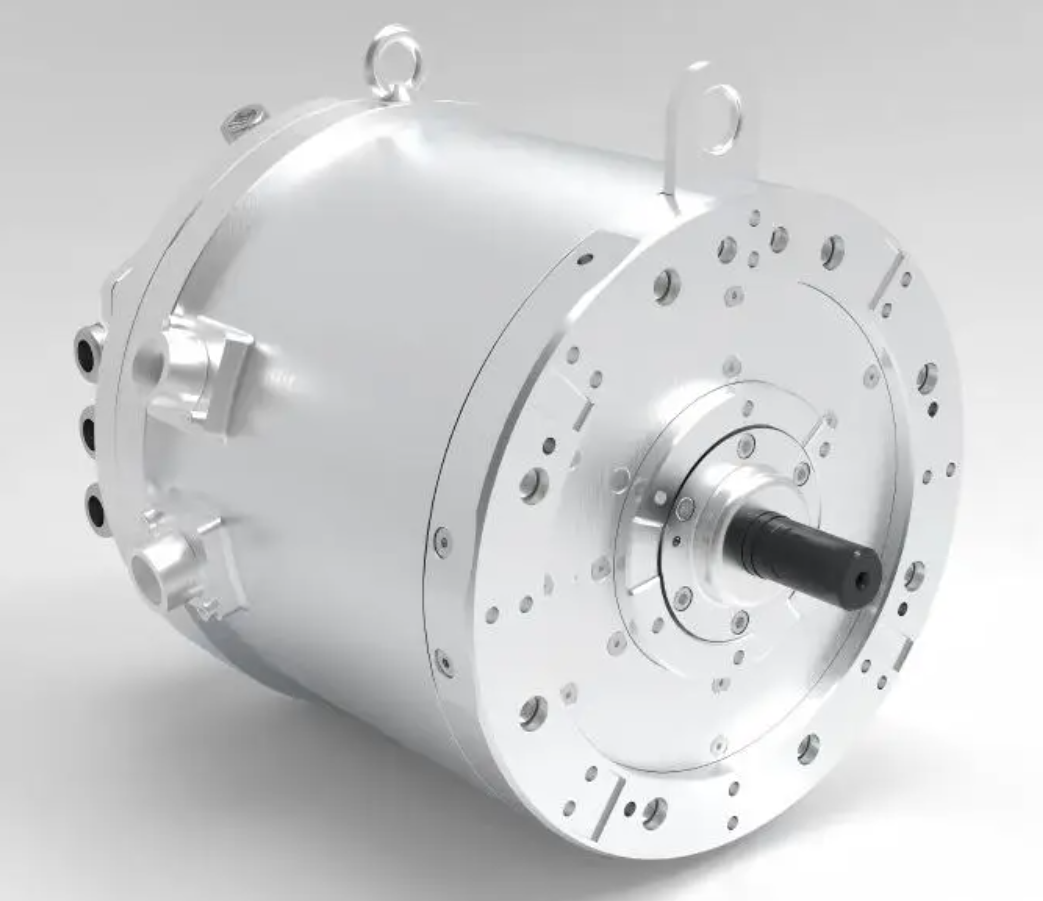
1. Electric-Vehicle Propulsion Context
I view the electric vehicle as an integrated energy and motion system. The traction permanent magnet synchronous motor is not an isolated component. It interacts with the battery, the inverter, the transmission, the vehicle controller, and the driver. The driver expresses intent through the accelerator pedal, brake pedal, and steering wheel. The vehicle controller translates that intent into torque or speed commands. The motor controller then converts those commands into switching signals for the inverter, which regulates the permanent magnet synchronous motor. Because the permanent magnet synchronous motor has nonlinear magnetic and electrical behavior, the control problem is not simply a matter of applying a fixed voltage-to-frequency ratio. I must account for the d-q axis coupling, the voltage limit imposed by the DC bus and modulation method, and the current limit imposed by the inverter and the permanent magnet synchronous motor winding.
In most driving conditions, I use torque control for the permanent magnet synchronous motor. In special modes such as cruise control, I use speed control. Therefore, a speed-current double closed-loop structure is often the most practical baseline for an electric-vehicle permanent magnet synchronous motor drive. The outer speed loop provides the desired speed tracking, while the inner current loops provide fast dynamic response and protect the permanent magnet synchronous motor and inverter from overcurrent. I extend this baseline with a voltage loop that performs flux weakening when the permanent magnet synchronous motor reaches the base speed.
| Subsystem | Main Components | Primary Function | Interaction with Permanent Magnet Synchronous Motor |
|---|---|---|---|
| Electric drive system | Permanent magnet synchronous motor, motor controller, power electronics, transmission | Convert electrical energy into mechanical torque and speed | Directly determines torque, speed, efficiency, and flux-weakening capability |
| Power supply system | Battery, energy management system, charger | Provide stable DC voltage and monitor energy usage | Sets DC bus voltage and therefore the maximum stator voltage available to the permanent magnet synchronous motor |
| Auxiliary system | Steering, braking, thermal management, comfort loads | Improve handling, stability, and passenger comfort | Indirectly affects available energy and thermal margin for the permanent magnet synchronous motor |
2. Mathematical Model of the Permanent Magnet Synchronous Motor
I establish the mathematical model of the permanent magnet synchronous motor in the synchronous rotating d-q reference frame. I neglect magnetic saturation, eddy-current loss, hysteresis loss, slotting, and armature reaction. These assumptions are acceptable for the first design and simulation stage, and they produce a model that is accurate enough to reveal the essential flux-weakening behavior of the permanent magnet synchronous motor. I define the d-axis as aligned with the rotor permanent magnet flux and the q-axis as ninety electrical degrees ahead. The voltage equations of the permanent magnet synchronous motor are as follows.
$$u_d = R_s i_d + L_d \frac{di_d}{dt} – \omega_e L_q i_q$$
$$u_q = R_s i_q + L_q \frac{di_q}{dt} + \omega_e \left( L_d i_d + \psi_f \right)$$
The flux-linkage equations of the permanent magnet synchronous motor are expressed as follows.
$$\psi_d = L_d i_d + \psi_f$$
$$\psi_q = L_q i_q$$
The electromagnetic torque equation of the permanent magnet synchronous motor is given by the following expression.
$$T_e = \frac{3}{2} n_p \left[ \psi_f i_q + \left( L_d – L_q \right) i_d i_q \right]$$
The mechanical motion equation of the permanent magnet synchronous motor and the connected drivetrain is written as follows.
$$J \frac{d\omega_m}{dt} = T_e – T_L – B \omega_m$$
The electrical angular speed and mechanical angular speed of the permanent magnet synchronous motor are related by the pole-pair number.
$$\omega_e = n_p \omega_m$$
The symbols used in the permanent magnet synchronous motor model are summarized below.
| Symbol | Meaning | Unit |
|---|---|---|
| \(u_d\) | d-axis stator voltage | V |
| \(u_q\) | q-axis stator voltage | V |
| \(i_d\) | d-axis stator current | A |
| \(i_q\) | q-axis stator current | A |
| \(R_s\) | Stator phase resistance | \(\Omega\) |
| \(L_d\) | d-axis inductance | H |
| \(L_q\) | q-axis inductance | H |
| \(\psi_f\) | Permanent magnet flux linkage | Wb |
| \(n_p\) | Pole-pair number | — |
| \(T_e\) | Electromagnetic torque | N·m |
| \(T_L\) | Load torque | N·m |
| \(J\) | Rotor and load inertia | kg·m² |
| \(B\) | Viscous damping coefficient | N·m·s/rad |
| \(\omega_m\) | Mechanical angular speed | rad/s |
| \(\omega_e\) | Electrical angular speed | rad/s |
Substituting the flux-linkage equations into the voltage equations and the torque equation into the motion equation yields the complete dynamic model of the permanent magnet synchronous motor. I observe that the d-axis and q-axis are coupled through the terms \(\omega_e L_q i_q\) and \(\omega_e (L_d i_d + \psi_f)\). This coupling is nonlinear, and it becomes more severe as the speed of the permanent magnet synchronous motor increases. For this reason, I include a decoupling block in the current control loops. Without decoupling, the current regulators must fight the back-electromotive-force terms, and the dynamic performance of the permanent magnet synchronous motor degrades in the high-speed region.
3. Voltage and Current Constraints
I now examine the constraints that make flux weakening necessary for the permanent magnet synchronous motor. The inverter has a finite DC bus voltage, and the modulation method determines the maximum fundamental stator voltage that can be synthesized without distortion. The permanent magnet synchronous motor winding and the inverter also have a maximum current rating. Therefore, the permanent magnet synchronous motor must obey both a voltage limit and a current limit.
Let the maximum available stator phase voltage be \(u_{s,\max}\). The voltage constraint of the permanent magnet synchronous motor is as follows.
$$u_d^2 + u_q^2 \le u_{s,\max}^2$$
Let the maximum available stator phase current be \(i_{s,\max}\). The current constraint of the permanent magnet synchronous motor is expressed as follows.
$$i_d^2 + i_q^2 \le i_{s,\max}^2$$
If I neglect the stator resistance and the transient inductance terms for steady-state analysis, the voltage constraint of the permanent magnet synchronous motor becomes the following elliptic relationship in the d-q current plane.
$$\left( L_d i_d + \psi_f \right)^2 + \left( L_q i_q \right)^2 \le \left( \frac{u_{s,\max}}{\omega_e} \right)^2$$
For a surface-mounted permanent magnet synchronous motor, where \(L_d = L_q = L\), the voltage constraint becomes a circle.
$$\left( i_d + \frac{\psi_f}{L} \right)^2 + i_q^2 \le \left( \frac{u_{s,\max}}{L \omega_e} \right)^2$$
The current constraint is always a circle centered at the origin.
$$i_d^2 + i_q^2 \le i_{s,\max}^2$$
I interpret these constraints as follows. The current limit circle is fixed. The voltage limit ellipse or circle shrinks as the electrical angular speed of the permanent magnet synchronous motor increases. At low speed, the voltage limit is wide, and the permanent magnet synchronous motor can produce high torque within the current limit. At high speed, the voltage limit becomes small, and the operating point must move along the current limit circle toward negative \(i_d\). This negative \(i_d\) weakens the rotor flux and allows the permanent magnet synchronous motor to continue operating at higher speed. The intersection of the voltage limit and current limit defines the feasible operating region of the permanent magnet synchronous motor.
| Constraint | Mathematical Form | Geometric Shape | Effect on Permanent Magnet Synchronous Motor |
|---|---|---|---|
| Voltage limit | \(u_d^2 + u_q^2 \le u_{s,\max}^2\) | Ellipse or circle in the d-q plane | Shrinks as speed increases and forces negative d-axis current |
| Current limit | \(i_d^2 + i_q^2 \le i_{s,\max}^2\) | Circle centered at origin | Sets maximum torque and maximum demagnetizing current |
| Thermal limit | \(i_s^2 = i_d^2 + i_q^2 \le i_{th}^2\) | Circle or derated current region | Protects permanent magnet synchronous motor winding insulation and magnets |
| DC bus limit | \(u_{s,\max} = U_{dc}/\sqrt{3}\) for linear SVPWM | Fixed voltage ceiling | Determines the base speed and the depth of flux weakening |
4. Operating Regions of the Permanent Magnet Synchronous Motor
I divide the speed range of the permanent magnet synchronous motor into three regions. This division helps me design a control strategy that is smooth and stable across the entire operating envelope. The first region is the constant-torque region below the base speed. The second region is the constant-power flux-weakening region between the base speed and the maximum torque per voltage speed. The third region is the deep flux-weakening region, which exists only when the characteristic current \(\psi_f/L_d\) is less than the maximum stator current \(i_{s,\max}\).
| Region | Speed Range | Main Control Objective | Current Trajectory | Permanent Magnet Synchronous Motor Behavior |
|---|---|---|---|---|
| Region I | \(\omega \le \omega_b\) | Maximum torque per ampere or zero d-axis current | Origin to point on current limit circle | Constant torque, high acceleration, good low-speed response |
| Region II | \(\omega_b \le \omega \le \omega_{mtpv}\) | Constant power with current-limited operation | Along current limit circle toward negative d-axis | Torque decreases as speed rises while power remains high |
| Region III | \(\omega_{mtpv} \le \omega \le \omega_{\max}\) | Maximum torque per voltage with voltage-limited operation | Along maximum torque per voltage curve | Deep flux weakening, very high speed, reduced torque capability |
In Region I, I can use \(i_d = 0\) control for a surface-mounted permanent magnet synchronous motor. This is simple and effective because the torque of a surface-mounted permanent magnet synchronous motor is proportional to \(i_q\). For an interior permanent magnet synchronous motor, I use maximum torque per ampere control because the reluctance torque term \((L_d – L_q)i_d i_q\) can improve efficiency. In both cases, the permanent magnet synchronous motor operates below the base speed, and the voltage limit is not active.
In Region II, the voltage limit becomes active. I must reduce the q-axis current and introduce negative d-axis current. The current vector moves along the current limit circle. The permanent magnet synchronous motor enters the constant-power region. The transition from Region I to Region II must be smooth; otherwise, the driver may feel a torque discontinuity. I design the advanced-angle flux-weakening controller to make this transition continuous.
In Region III, the voltage limit dominates. The current vector follows the maximum torque per voltage trajectory. The permanent magnet synchronous motor is deeply flux weakened. The available torque decreases rapidly with speed, but the speed range is extended. This region is important for high-speed overtaking and high-speed cruising, even though the permanent magnet synchronous motor cannot produce full torque there.
5. Maximum Torque per Ampere and Maximum Torque per Voltage
I use maximum torque per ampere control in the low-speed region to obtain the largest torque for a given stator current. For an interior permanent magnet synchronous motor, the maximum torque per ampere condition is derived by expressing the current vector in terms of the current angle. I define the current angle \(\beta\) as the angle between the stator current vector and the q-axis.
$$i_d = -i_s \sin\beta$$
$$i_q = i_s \cos\beta$$
Substituting these expressions into the torque equation of the permanent magnet synchronous motor gives the following.
$$T_e = \frac{3}{2} n_p \left[ \psi_f i_s \cos\beta + \frac{1}{2} \left( L_q – L_d \right) i_s^2 \sin 2\beta \right]$$
For an interior permanent magnet synchronous motor, I solve for the maximum torque per ampere condition by differentiating the torque with respect to \(\beta\) and setting the derivative to zero. The resulting d-axis current reference is as follows.
$$i_d^{mtpa} = \frac{-\psi_f + \sqrt{\psi_f^2 + 4 \left( L_q – L_d \right)^2 i_q^2}}{2 \left( L_q – L_d \right)}$$
For a surface-mounted permanent magnet synchronous motor, \(L_d = L_q\), so the maximum torque per ampere condition simplifies to \(i_d = 0\). The torque equation of the surface-mounted permanent magnet synchronous motor becomes the following.
$$T_e = \frac{3}{2} n_p \psi_f i_q$$
In the high-speed region, I use maximum torque per voltage control. The maximum torque per voltage trajectory is the locus of operating points that produce the maximum torque for a given voltage limit. It is obtained by combining the torque equation of the permanent magnet synchronous motor with the voltage limit equation and solving for the current vector that maximizes torque. The maximum torque per voltage condition is especially important in Region III, where the voltage limit is the active constraint. For a surface-mounted permanent magnet synchronous motor, the maximum torque per voltage trajectory requires negative \(i_d\) according to the following voltage-limited relationship.
$$i_d^{fw} = -\frac{\psi_f}{L} + \frac{1}{L} \sqrt{\left( \frac{u_{s,\max}}{\omega_e} \right)^2 – \left( L i_q \right)^2}$$
This equation shows that as the electrical angular speed of the permanent magnet synchronous motor increases, the allowable positive q-axis current decreases, and the required negative d-axis current becomes more negative. In other words, the permanent magnet synchronous motor must be flux weakened more deeply at higher speed.
| Control Method | Region of Use | Main Advantage | Main Limitation | Effect on Permanent Magnet Synchronous Motor |
|---|---|---|---|---|
| \(i_d = 0\) | Low-speed surface PMSM | Simple, high torque per ampere for surface PMSM | No reluctance torque, poor high-speed capability | Keeps permanent magnet synchronous motor in constant-torque mode |
| Maximum torque per ampere | Low-speed interior PMSM | Minimum copper loss for given torque | Requires accurate inductance parameters | Improves efficiency of permanent magnet synchronous motor |
| Formula-based flux weakening | Medium-speed region | Easy to implement | High parameter sensitivity | Can cause torque error in permanent magnet synchronous motor |
| Lookup-table flux weakening | Calibrated operating range | Good steady-state accuracy | Large calibration effort, poor adaptability | Requires extensive testing of permanent magnet synchronous motor |
| Gradient flux weakening | High-speed region | Good dynamic response | Complex computation | Improves voltage utilization of permanent magnet synchronous motor |
| Negative \(i_d\) compensation | High-speed region | Simple structure | Stability problems in deep flux weakening | Can cause current oscillation in permanent magnet synchronous motor |
| Advanced-angle flux weakening | Full speed range | Smooth transition, good stability, wide speed range | Requires voltage loop tuning | Enables safe high-speed operation of permanent magnet synchronous motor |
6. Proposed Advanced-Angle Flux-Weakening Control Strategy
I propose an advanced-angle flux-weakening control strategy for the permanent magnet synchronous motor. The central idea is to regulate the phase angle of the stator current vector so that the voltage limit is respected without abrupt changes in the torque command. I define the advanced angle \(\gamma\) as the angle by which the stator current vector is shifted relative to the q-axis. When \(\gamma = 0\), the stator current is entirely on the q-axis, and the permanent magnet synchronous motor operates in the non-flux-weakening mode. When \(\gamma < 0\), the stator current has a negative d-axis component, and the permanent magnet synchronous motor enters flux weakening. The current components are as follows.
$$i_d = i_s \sin\gamma$$
$$i_q = i_s \cos\gamma$$
Because \(\gamma\) is negative during flux weakening, \(i_d\) is negative. The negative d-axis current produces a flux that opposes the permanent magnet flux. This reduces the effective flux linkage of the permanent magnet synchronous motor and allows the voltage constraint to be satisfied at a higher speed.
My control structure includes an outer speed loop, an inner d-axis current loop, an inner q-axis current loop, and a voltage loop. The speed loop generates the torque or q-axis current reference. The voltage loop monitors the stator voltage magnitude. If the required voltage exceeds the maximum available voltage, the voltage loop reduces the advanced angle, which increases the negative d-axis current and weakens the permanent magnet flux. If the required voltage is below the limit, the voltage loop allows the advanced angle to return toward zero, which reduces the negative d-axis current and improves efficiency.
I express the voltage loop as a proportional-integral controller with saturation. The voltage magnitude of the permanent magnet synchronous motor is calculated from the d-axis and q-axis voltage references.
$$u_s^{ref} = \sqrt{ \left( u_d^{ref} \right)^2 + \left( u_q^{ref} \right)^2 }$$
The voltage error is defined as follows.
$$\Delta u = u_{s,\max} – u_s^{ref}$$
The advanced angle is then generated by the following control law.
$$\gamma = \operatorname{sat} \left( K_{p,u} \Delta u + K_{i,u} \int \Delta u \, dt, -\frac{\pi}{2}, 0 \right)$$
The saturation function ensures that the advanced angle remains within the permissible flux-weakening range. When the voltage error is positive, meaning that the available voltage is greater than the required voltage, the integrator can increase \(\gamma\) toward zero. When the voltage error is negative, meaning that the required voltage exceeds the available voltage, the controller drives \(\gamma\) negative. This produces negative \(i_d\) and reduces the voltage demand of the permanent magnet synchronous motor.
The current references are generated from the advanced angle and the stator current magnitude reference.
$$i_d^* = i_s^* \sin\gamma$$
$$i_q^* = i_s^* \cos\gamma$$
I also apply current limiting to protect the permanent magnet synchronous motor and the inverter.
$$i_d^* = \max \left( i_d^*, -i_{s,\max} \right)$$
$$i_q^* = \operatorname{sign} \left( i_q^* \right) \min \left( \left| i_q^* \right|, \sqrt{ i_{s,\max}^2 – \left( i_d^* \right)^2 } \right)$$
To improve the dynamic performance of the permanent magnet synchronous motor, I add feedforward decoupling to the current loops. The decoupling terms cancel the cross-coupling in the permanent magnet synchronous motor voltage equations.
$$u_d^{dec} = u_d^{PI} – \omega_e L_q i_q$$
$$u_q^{dec} = u_q^{PI} + \omega_e \left( L_d i_d + \psi_f \right)$$
The compensated voltage commands are then passed to the space-vector pulse-width modulation block. For linear modulation, the maximum fundamental phase voltage is related to the DC bus voltage by the following expression.
$$u_{s,\max} = \frac{U_{dc}}{\sqrt{3}}$$
When the permanent magnet synchronous motor operates below the base speed, the voltage loop is positively saturated, the advanced angle is zero, and the permanent magnet synchronous motor operates in the constant-torque mode. When the permanent magnet synchronous motor exceeds the base speed, the voltage loop leaves saturation, the advanced angle becomes negative, and the permanent magnet synchronous motor enters the constant-power flux-weakening mode. This transition is smooth because the voltage loop adjusts the advanced angle continuously.
| Control Loop | Input | Output | Purpose | Benefit for Permanent Magnet Synchronous Motor |
|---|---|---|---|---|
| Speed loop | Speed error | Torque or q-axis current reference | Track driver speed demand | Provides high-precision speed regulation of permanent magnet synchronous motor |
| d-axis current loop | \(i_d\) error | \(u_d\) command | Regulate flux-producing current | Controls flux weakening of permanent magnet synchronous motor |
| q-axis current loop | \(i_q\) error | \(u_q\) command | Regulate torque-producing current | Controls torque of permanent magnet synchronous motor |
| Voltage loop | Voltage error | Advanced angle \(\gamma\) | Prevent voltage saturation | Extends speed range of permanent magnet synchronous motor |
| Decoupling block | \(i_d\), \(i_q\), \(\omega_e\) | Feedforward voltage terms | Cancel d-q coupling | Improves dynamic response of permanent magnet synchronous motor |
7. Design Procedure for the Proposed Controller
I follow a systematic procedure when I design the advanced-angle flux-weakening controller for the permanent magnet synchronous motor. First, I identify the machine parameters: stator resistance, d-axis inductance, q-axis inductance, permanent magnet flux linkage, pole-pair number, rated current, rated torque, and maximum speed. Second, I determine the DC bus voltage and the modulation limit. Third, I calculate the base speed of the permanent magnet synchronous motor. Fourth, I tune the current loops with decoupling. Fifth, I tune the voltage loop so that the advanced angle responds quickly but does not oscillate. Sixth, I verify the controller in simulation and then on a dynamometer.
I calculate the base speed of the permanent magnet synchronous motor from the voltage limit and the rated operating point. In the constant-torque region, I assume \(i_d = 0\) for a surface-mounted permanent magnet synchronous motor. The q-axis voltage at the base speed satisfies the following approximate relationship.
$$u_{s,\max}^2 = \left( R_s i_q \right)^2 + \left( \omega_{e,b} \psi_f + \omega_{e,b} L_d i_d \right)^2$$
If I neglect the resistive drop and set \(i_d = 0\), the base electrical angular speed of the permanent magnet synchronous motor is approximately as follows.
$$\omega_{e,b} \approx \frac{u_{s,\max}}{\psi_f}$$
The corresponding base mechanical speed is obtained from the pole-pair number.
$$\omega_{m,b} = \frac{\omega_{e,b}}{n_p}$$
This estimate shows that the base speed of the permanent magnet synchronous motor is inversely proportional to the permanent magnet flux linkage. A stronger magnet gives higher torque but lower base speed. Flux weakening is therefore essential when I want a wide constant-power speed range from a permanent magnet synchronous motor with a high flux linkage.
| Design Step | Action | Key Equation or Criterion | Reason |
|---|---|---|---|
| 1 | Collect permanent magnet synchronous motor parameters | \(R_s, L_d, L_q, \psi_f, n_p, i_{s,\max}, \omega_{\max}\) | Provides model basis |
| 2 | Determine DC bus and voltage limit | \(u_{s,\max} = U_{dc}/\sqrt{3}\) | Sets achievable voltage |
| 3 | Estimate base speed | \(\omega_{e,b} \approx u_{s,\max}/\psi_f\) | Identifies flux-weakening onset |
| 4 | Tune current loops | Bandwidth, phase margin, decoupling gains | Ensures fast torque response |
| 5 | Tune voltage loop | \(K_{p,u}, K_{i,u}\), saturation limits | Ensures smooth flux weakening |
| 6 | Validate in simulation | Step speed, step load, full-speed sweep | Checks stability and transition |
| 7 | Validate experimentally | Dynamometer, thermal test, efficiency map | Confirms practical performance |
8. Simulation Model and Validation
I build a simulation model of the electric-vehicle permanent magnet synchronous motor drive in MATLAB/Simulink. The model includes the permanent magnet synchronous motor, the inverter, the space-vector pulse-width modulation block, the speed controller, the current controllers, the decoupling block, and the advanced-angle flux-weakening controller. I set the DC bus voltage to 800 V. I set the initial target speed to 8000 r/min and the load torque to 70 N·m. At 0.5 s, I increase the target speed to 14000 r/min. At 1.0 s, I increase the target speed to 18000 r/min. I record the motor speed, voltage vector magnitude, advanced angle, and d-axis current.
| Parameter | Value | Unit |
|---|---|---|
| DC bus voltage | 800 | V |
| Initial target speed | 8000 | r/min |
| Second target speed | 14000 | r/min |
| Third target speed | 18000 | r/min |
| Load torque | 70 | N·m |
| Speed step time 1 | 0.5 | s |
| Speed step time 2 | 1.0 | s |
I observe that from 0 to 0.5 s, the permanent magnet synchronous motor operates below its base speed. The stator voltage vector magnitude remains below the voltage limit. The advanced angle is zero radians, and the d-axis current is zero amperes. The permanent magnet synchronous motor is in the non-flux-weakening state. The speed loop and current loops track the command accurately, and the torque response is fast.
From 0.5 to 1.0 s, the permanent magnet synchronous motor exceeds the base speed. The stator voltage would exceed the voltage limit if no flux weakening were applied. The voltage loop activates, and the advanced angle becomes negative. This produces a negative d-axis current, which weakens the rotor flux. The permanent magnet synchronous motor remains stable in the high-speed flux-weakening region. The voltage vector magnitude is held near its maximum, and the current vector rotates toward the negative d-axis.
From 1.0 to 1.5 s, the permanent magnet synchronous motor speed increases further. The voltage limit continues to tighten. The advanced angle becomes more negative, and the d-axis current becomes more negative. The permanent magnet synchronous motor maintains high-speed operation even though the available torque is reduced. The transition between the constant-torque region and the flux-weakening region is smooth. I do not observe severe torque ripple or speed oscillation. The simulation results confirm that the proposed advanced-angle flux-weakening control strategy can extend the speed range of the permanent magnet synchronous motor and keep the drive stable across multiple operating regions.
| Time Interval | Speed Condition | Advanced Angle | d-Axis Current | Voltage Condition | Permanent Magnet Synchronous Motor State |
|---|---|---|---|---|---|
| 0–0.5 s | Below base speed | 0 rad | 0 A | Below limit | Constant-torque, non-flux-weakening |
| 0.5–1.0 s | Above base speed | Negative | Negative | At or near limit | Constant-power flux weakening |
| 1.0–1.5 s | Deep high speed | More negative | More negative | At limit | Deep flux weakening |
9. Stability and Parameter Sensitivity
I pay close attention to stability because flux weakening can push the permanent magnet synchronous motor toward the edge of the feasible operating region. The voltage loop must be tuned so that it does not interact adversely with the current loops. If the voltage loop is too fast, it can cause oscillation in the advanced angle and the d-axis current. If it is too slow, the permanent magnet synchronous motor may momentarily exceed the voltage limit during fast acceleration. I therefore choose the voltage loop bandwidth to be lower than the current loop bandwidth but high enough to track speed transients.
Parameter sensitivity is another important issue for the permanent magnet synchronous motor. The d-axis inductance, q-axis inductance, and permanent magnet flux linkage vary with temperature, current level, and magnetic saturation. If the controller relies on a fixed mathematical formula for flux weakening, errors in these parameters can cause incorrect d-axis current and reduced torque accuracy. My advanced-angle strategy reduces this sensitivity because it uses voltage feedback rather than a pure feedforward formula. The voltage loop automatically increases the negative d-axis current when the voltage limit is approached, even if the machine parameters change. This feedback action makes the permanent magnet synchronous motor more robust in real driving conditions.
| Parameter | Variation Source | Effect on Permanent Magnet Synchronous Motor | Mitigation in Advanced-Angle Control |
|---|---|---|---|
| \(\psi_f\) | Temperature, magnet aging | Changes base speed and flux-weakening depth | Voltage feedback compensates automatically |
| \(L_d\) | Saturation, current level | Changes voltage limit ellipse and d-axis current requirement | Closed-loop voltage regulation reduces sensitivity |
| \(L_q\) | Saturation, cross-coupling | Changes torque and voltage coupling | Feedforward decoupling and current feedback |
| \(R_s\) | Temperature | Changes copper loss and voltage drop | Current loop integral action compensates |
| \(U_{dc}\) | Battery state of charge, load | Changes maximum available voltage | Voltage loop uses measured DC bus voltage |
10. Implementation Considerations for Electric Vehicles
I consider several practical issues when I move the permanent magnet synchronous motor controller from simulation to an embedded electric-vehicle platform. First, the voltage loop must use the measured or estimated stator voltage, not the commanded voltage alone, because inverter dead time, device voltage drop, and DC bus variation introduce errors. Second, the current sampling must be synchronized with the pulse-width modulation to avoid switching noise. Third, the advanced angle must be limited to prevent excessive demagnetizing current that could permanently damage the magnets of the permanent magnet synchronous motor. Fourth, the controller must coordinate with the battery management system so that deep flux weakening is allowed only when the DC bus can supply the required current without excessive voltage sag.
I also consider thermal management. Flux weakening increases the d-axis current, which does not produce torque in a surface-mounted permanent magnet synchronous motor. This current causes copper loss and reduces efficiency. Therefore, I use flux weakening only when necessary. In the low-speed region, I keep \(i_d\) near zero or at the maximum torque per ampere value. In the high-speed region, I allow negative \(i_d\) to maintain voltage control. The energy management system can use the efficiency map of the permanent magnet synchronous motor to decide how aggressively to flux weaken during cruising. If the driver demands high torque at high speed, the controller must prioritize torque. If the driver demands efficient cruising, the controller can choose a more efficient operating point within the feasible region.
| Implementation Issue | Risk | Countermeasure | Impact on Permanent Magnet Synchronous Motor |
|---|---|---|---|
| Inverter dead time | Voltage distortion and current error | Dead-time compensation | Improves voltage accuracy for permanent magnet synchronous motor |
| Current sampling noise | Torque ripple and unstable current loop | Synchronized sampling and filtering | Protects permanent magnet synchronous motor from current spikes |
| Magnet demagnetization | Permanent loss of torque | Current limit and thermal protection | Ensures long-term health of permanent magnet synchronous motor |
| DC bus variation | Voltage limit uncertainty | Real-time DC bus measurement | Maintains stable flux weakening of permanent magnet synchronous motor |
| Parameter drift | Torque error and efficiency loss | Online estimation or robust feedback | Keeps permanent magnet synchronous motor operating near desired point |
11. Comparison with Conventional Flux-Weakening Methods
I compare the proposed advanced-angle method with conventional flux-weakening methods for the permanent magnet synchronous motor. The formula method uses a direct equation to calculate the d-axis current from speed and torque. It is simple, but it depends heavily on machine parameters. The lookup-table method uses calibrated data and can achieve good steady-state accuracy, but it requires extensive testing and cannot easily adapt to parameter drift. The gradient method uses optimization or search to find the operating point, which can be accurate but computationally expensive. The negative \(i_d\) compensation method is simple but can suffer from poor stability in deep flux weakening. My advanced-angle method uses voltage feedback to generate the current angle, so it combines simplicity with robustness. It also provides smooth transitions between the constant-torque and constant-power regions.
| Method | Parameter Sensitivity | Steady-State Accuracy | Dynamic Response | Deep Flux-Weakening Stability | Implementation Complexity |
|---|---|---|---|---|---|
| Formula method | High | Medium | Medium | Medium | Low |
| Lookup table | Medium | High | Medium | Medium | High calibration |
| Gradient method | Low | High | High | High | High |
| Negative \(i_d\) compensation | High | Medium | Medium | Low | Low |
| Advanced-angle method | Low to medium | High | High | High | Medium |
12. Extended Discussion of Voltage-Limited Operation
I now derive additional relationships that help me understand the voltage-limited operation of the permanent magnet synchronous motor. In steady state, I neglect the stator resistance and the derivative terms. The voltage equations of the permanent magnet synchronous motor reduce to the following.
$$u_d = -\omega_e L_q i_q$$
$$u_q = \omega_e \left( L_d i_d + \psi_f \right)$$
The stator voltage magnitude is therefore as follows.
$$u_s^2 = \omega_e^2 \left[ \left( L_q i_q \right)^2 + \left( L_d i_d + \psi_f \right)^2 \right]$$
At the voltage limit, I obtain the voltage constraint equation of the permanent magnet synchronous motor.
$$\left( L_q i_q \right)^2 + \left( L_d i_d + \psi_f \right)^2 = \left( \frac{u_{s,\max}}{\omega_e} \right)^2$$
For a surface-mounted permanent magnet synchronous motor, \(L_d = L_q = L\). The voltage constraint becomes the following circle.
$$\left( i_d + \frac{\psi_f}{L} \right)^2 + i_q^2 = \left( \frac{u_{s,\max}}{L \omega_e} \right)^2$$
The center of this voltage-limit circle is at \(-\psi_f/L\), and the radius is \(u_{s,\max}/(L\omega_e)\). As the speed increases, the radius decreases. The current limit circle is centered at the origin with radius \(i_{s,\max}\). The feasible region of the permanent magnet synchronous motor is the intersection of these two circles. When the voltage-limit circle no longer intersects the current-limit circle at a positive \(i_q\), the permanent magnet synchronous motor must reduce torque and increase negative \(i_d\). This is the fundamental reason why flux weakening is necessary.
I can also define the characteristic current of the permanent magnet synchronous motor as follows.
$$i_{ch} = \frac{\psi_f}{L}$$
If \(i_{ch} \le i_{s,\max}\), the permanent magnet synchronous motor can theoretically be operated at infinite speed with zero torque, because the voltage-limit circle can be centered inside the current-limit circle. If \(i_{ch} > i_{s,\max}\), the permanent magnet synchronous motor has a finite maximum speed even with maximum demagnetizing current. This distinction is important when I select a permanent magnet synchronous motor for an electric vehicle. I prefer a machine with a characteristic current close to or below the inverter current limit so that a wide constant-power speed range is achievable.
| Condition | Geometric Interpretation | Speed Capability of Permanent Magnet Synchronous Motor | Design Implication |
|---|---|---|---|
| \(i_{ch} < i_{s,\max}\) | Voltage-limit circle center inside current-limit circle | Theoretically infinite speed with zero torque | Wide speed range, good for traction |
| \(i_{ch} = i_{s,\max}\) | Voltage-limit circle center on current-limit circle | Very wide speed range | Balanced design |
| \(i_{ch} > i_{s,\max}\) | Voltage-limit circle center outside current-limit circle | Finite maximum speed | Limited flux-weakening capability |
13. Torque and Power Characteristics
I summarize the torque and power characteristics of the permanent magnet synchronous motor under the proposed control strategy. In the constant-torque region, the torque is limited by the current limit. The power increases linearly with speed. In the constant-power region, the torque decreases inversely with speed. The power remains approximately constant until the voltage limit becomes the dominant constraint. In the deep flux-weakening region, the torque decreases more rapidly, and the power may decline if the current limit and voltage limit cannot maintain constant power.
| Region | Torque Behavior | Power Behavior | Current Limit Active? | Voltage Limit Active? |
|---|---|---|---|---|
| Constant torque | Constant maximum torque | Increases linearly with speed | Yes | No |
| Constant power | Decreases inversely with speed | Approximately constant | Yes | Yes, increasingly |
| Deep flux weakening | Decreases rapidly | May decrease | Sometimes | Yes |
The transition between the constant-torque and constant-power regions occurs at the base speed of the permanent magnet synchronous motor. I can shift this base speed by changing the DC bus voltage, the permanent magnet flux linkage, or the number of pole pairs. In an electric vehicle, the DC bus voltage is often fixed by the battery pack, so the base speed is mainly determined by the machine design. If I need a higher base speed, I can reduce the permanent magnet flux linkage, but this reduces the low-speed torque. Thus, there is a trade-off between low-speed torque and high-speed range. Flux weakening is the control-level solution that allows a machine with high low-speed torque to also achieve a high maximum speed.
14. Advanced Angle and Current Vector Trajectory
I further analyze the current vector trajectory of the permanent magnet synchronous motor under advanced-angle control. The current magnitude is limited by the current limit circle. The current angle \(\gamma\) determines how much of the current is used for flux weakening. When \(\gamma = 0\), the current is entirely on the q-axis. When \(\gamma = -\pi/2\), the current is entirely on the negative d-axis and produces no torque in a surface-mounted permanent magnet synchronous motor. In practice, I limit \(\gamma\) to a value that preserves torque production and protects the magnets. The current vector trajectory moves from the positive q-axis toward the negative d-axis as speed increases.
I can express the torque of a surface-mounted permanent magnet synchronous motor as a function of the advanced angle.
$$T_e = \frac{3}{2} n_p \psi_f i_s \cos\gamma$$
For an interior permanent magnet synchronous motor, the torque includes the reluctance term.
$$T_e = \frac{3}{2} n_p \left[ \psi_f i_s \cos\gamma + \frac{1}{2} \left( L_q – L_d \right) i_s^2 \sin 2\gamma \right]$$
These expressions show that the torque decreases as the advanced angle becomes more negative. The controller must therefore balance the need for voltage reduction against the need for torque production. The voltage loop does this automatically by adjusting \(\gamma\) until the voltage constraint is satisfied.
15. Simulation Results and Interpretation
I interpret the simulation results in terms of the physical behavior of the permanent magnet synchronous motor. The speed waveform shows that the permanent magnet synchronous motor tracks the commanded speed steps without significant overshoot. The voltage vector magnitude waveform shows that the voltage rises with speed until it reaches the limit. After that point, the voltage remains at the limit while the advanced angle becomes negative. The advanced angle waveform shows a smooth transition from zero to negative values. The d-axis current waveform shows a smooth transition from zero to negative values. These waveforms confirm that the voltage loop is performing flux weakening correctly and that the permanent magnet synchronous motor remains stable.
I also examine the current limit. The total stator current remains within the maximum current rating. The q-axis current decreases as the d-axis current becomes more negative. The torque-producing current is reduced, but the permanent magnet synchronous motor can still operate at high speed. This is the expected behavior of a voltage-limited permanent magnet synchronous motor in the flux-weakening region.
| Observed Quantity | Low-Speed Behavior | High-Speed Behavior | Interpretation |
|---|---|---|---|
| Speed | Tracks command accurately | Tracks command accurately in flux weakening | Speed loop remains stable |
| Voltage magnitude | Below limit | At limit | Voltage loop active |
| Advanced angle | Zero | Negative | Flux weakening engaged |
| d-axis current | Zero or near zero | Negative | Rotor flux weakened |
| q-axis current | High | Reduced | Torque reduced at high speed |
16. Practical Tuning Guidelines
I recommend the following tuning guidelines for the advanced-angle flux-weakening controller of the permanent magnet synchronous motor. First, tune the current loops with a bandwidth at least five times higher than the speed loop. Second, include the decoupling terms before tuning the current loops, or account for them in the plant model. Third, tune the voltage loop with a bandwidth lower than the current loops but high enough to respond within the speed transient. Fourth, set the advanced angle saturation to a safe value based on the demagnetization limit of the permanent magnet synchronous motor. Fifth, test the controller with DC bus voltage variations, load steps, and speed reversals. Sixth, verify that the flux-weakening transition is smooth at the base speed and at the maximum torque per voltage speed.
| Tuning Parameter | Recommended Relationship | Reason | Effect on Permanent Magnet Synchronous Motor |
|---|---|---|---|
| Current loop bandwidth | \(\omega_{c,i} \gg \omega_{c,s}\) | Separate time scales | Fast torque response |
| Voltage loop bandwidth | \(\omega_{c,u} < \omega_{c,i}\) | Avoid interaction | Smooth flux weakening |
| Speed loop bandwidth | \(\omega_{c,s} < \omega_{c,u}\) | Stable speed control | Good driveability |
| Advanced angle limit | \(\gamma_{\min} > -\pi/2\) | Prevent pure demagnetization | Protects magnets |
| Current limit | \(i_s \le i_{s,\max}\) | Protect inverter and winding | Prevents overheating |
17. Summary of Equations
I provide a consolidated summary of the key equations used in the analysis and control of the permanent magnet synchronous motor.
| Description | Equation |
|---|---|
| d-axis voltage | \(u_d = R_s i_d + L_d \frac{di_d}{dt} – \omega_e L_q i_q\) |
| q-axis voltage | \(u_q = R_s i_q + L_q \frac{di_q}{dt} + \omega_e \left( L_d i_d + \psi_f \right)\) |
| d-axis flux linkage | \(\psi_d = L_d i_d + \psi_f\) |
| q-axis flux linkage | \(\psi_q = L_q i_q\) |
| Electromagnetic torque | \(T_e = \frac{3}{2} n_p \left[ \psi_f i_q + \left( L_d – L_q \right) i_d i_q \right]\) |
| Mechanical motion | \(J \frac{d\omega_m}{dt} = T_e – T_L – B \omega_m\) |
| Voltage limit | \(u_d^2 + u_q^2 \le u_{s,\max}^2\) |
| Current limit | \(i_d^2 + i_q^2 \le i_{s,\max}^2\) |
| Voltage ellipse | \(\left( L_d i_d + \psi_f \right)^2 + \left( L_q i_q \right)^2 \le \left( \frac{u_{s,\max}}{\omega_e} \right)^2\) |
| Advanced angle current components | \(i_d = i_s \sin\gamma, \quad i_q = i_s \cos\gamma\) |
| Voltage loop error | \(\Delta u = u_{s,\max} – u_s^{ref}\) |
| Advanced angle control law | \(\gamma = \operatorname{sat} \left( K_{p,u} \Delta u + K_{i,u} \int \Delta u \, dt, -\frac{\pi}{2}, 0 \right)\) |
| Maximum torque per ampere | \(i_d^{mtpa} = \frac{-\psi_f + \sqrt{\psi_f^2 + 4 \left( L_q – L_d \right)^2 i_q^2}}{2 \left( L_q – L_d \right)}\) |
| Flux-weakening current for surface PMSM | \(i_d^{fw} = -\frac{\psi_f}{L} + \frac{1}{L} \sqrt{\left( \frac{u_{s,\max}}{\omega_e} \right)^2 – \left( L i_q \right)^2}\) |
| Characteristic current | \(i_{ch} = \frac{\psi_f}{L}\) |
| Maximum linear SVPWM voltage | \(u_{s,\max} = \frac{U_{dc}}{\sqrt{3}}\) |
18. Conclusion
I have presented a comprehensive study of flux-weakening control for the permanent magnet synchronous motor in electric-vehicle traction applications. I began with the electric-vehicle system context and explained why the permanent magnet synchronous motor is a strong candidate for the traction drive. I then developed the mathematical model of the permanent magnet synchronous motor in the d-q reference frame, including the voltage, flux-linkage, torque, and motion equations. I analyzed the voltage and current constraints and showed how the voltage limit shrinks with speed, making flux weakening necessary. I divided the operating range into three regions and discussed the control objectives in each region. I proposed an advanced-angle flux-weakening control strategy that uses a voltage loop to adjust the phase angle of the stator current vector. This strategy provides smooth transitions between the constant-torque and constant-power regions, reduces parameter sensitivity, and maintains stability in deep flux weakening. I validated the method in MATLAB/Simulink with speed steps from 8000 r/min to 14000 r/min and then to 18000 r/min. The simulation results show that the permanent magnet synchronous motor tracks speed accurately, the voltage vector remains within the limit, the advanced angle becomes negative as required, and the d-axis current weakens the rotor flux to extend the speed range. I conclude that the proposed advanced-angle flux-weakening control strategy is a practical and effective solution for improving the high-speed performance of the permanent magnet synchronous motor in electric vehicles. It supports wide-speed operation, protects the permanent magnet synchronous motor from voltage saturation, and provides a solid foundation for further optimization of electric-vehicle drivetrains.